AGÕæÈË°Ù¼ÒÀÖ¹Ù·½ÍøÕ¾

First, let's import the required Python packages.

import os
import ee
import geemap

In order to use Earth Engine from within this Jupyter Notebook, we need to first Authenticate (which requires generating a token) and Initialize, as below. For more detailed instructions on the Authentication process, please refer to the: .

ee.Authenticate()

    To authorize access needed by Earth Engine, open the following URL in a web browser and follow the instructions:

    The authorization workflow will generate a code, which you should paste in the box below.

    Enter verification code:  

When you've entered the code, you should see the message:

    Successfully saved authorization token.

Once you've successfully authorized GEE, you can initialize as follows:

ee.Initialize()

First let's take a look at the available reflectance datasets - these come in 2 varieties: directional, and bidirectional. The bidirectional reflectance data have Bidirectional Reflectance Distribution Function (BRDF) and topographic corrections applied. The next few chunks of code show how you can do some initial data exploration, and determine what sites and how many years of data are available per site.

# Read in the NEON AOP Surface Directional Reflectance (HSI_REFL/001) Collection:
refl001 = ee.ImageCollection('projects/neon-prod-earthengine/assets/HSI_REFL/001')

# Read in the NEON AOP Surface Bidirectional Reflectance (HSI_REFL/002) Collection:
refl002 = ee.ImageCollection('projects/neon-prod-earthengine/assets/HSI_REFL/002')

# Determine available images in the NEON directional reflectance image collection:
refl001_list = refl001.aggregate_array('system:index').getInfo()
print('Available NEON Directional Reflectance Images:')
print(f'{len(refl001_list)} images available from the directional reflectance image collection')
print('first 10 images:')
print(refl001_list[:10])

# Determine available images in the NEON bidirectional reflectance image collection:
refl002_list = refl002.aggregate_array('system:index').getInfo()
print('\nAvailable NEON Bidirectional Reflectance Images:')
print(f'{len(refl002_list)} images available from the bidirectional reflectance image collection')
print('first 10 images:')
print(refl002_list[:10])

Available NEON Directional Reflectance Images:
61 images available from the directional reflectance image collection
first 10 images:
['2013_CPER_1', '2014_HARV_2', '2014_JERC_1', '2015_MLBS_1', '2015_TALL_1', '2016_CLBJ_1', '2016_GRSM_2', '2016_HARV_3', '2016_JERC_2', '2016_SERC_1']

Available NEON Bidirectional Reflectance Images:
68 images available from the bidirectional reflectance image collection
first 10 images:
['2022_ABBY_5', '2022_ARIK_4', '2022_BART_6', '2022_BLAN_5', '2022_CHEQ_7', '2022_CLBJ_6', '2022_CUPE_2', '2022_GUAN_2', '2022_GUIL_2', '2022_HOPB_4']

There are over 60 images in the directional and bidirectional reflectance image collections as of January 2025. Bidirectional data are currently only available for data collected between 2022-2024. More data for earlier years of data will be added in 2025, or you can request data for older directional reflectance data to be added if there is a site you would like to work with sooner. For this exercise, we will start by showing an example of the directional reflectance data since there currently is a longer archive of data available for that data product, but you would handle the bidirectional reflectance data the same way.

# Get the flight year and site information
refl001_years = refl001.aggregate_array('FLIGHT_YEAR').getInfo()
refl001_sites = refl001.aggregate_array('NEON_SITE').getInfo()
unique_refl001_sites = list(set(refl001_sites))
unique_refl001_sites.sort()
print('NEON sites included in the directional reflectance collection: \n', unique_refl001_sites)
print('NEON years included in the directional reflectance collection: \n', list(set(refl001_years)))
# print('NEON flight years included in the directional reflectance collection: \n', list(set(flightYears)))

# Get the flight year and site information
refl002_years = refl002.aggregate_array('FLIGHT_YEAR').getInfo()
refl002_sites = refl002.aggregate_array('NEON_SITE').getInfo()
unique_refl002_sites = list(set(refl002_sites))
unique_refl002_sites.sort()
print('\nNEON sites included in the bidirectional reflectance collection: \n', unique_refl002_sites)
print('NEON years included in the bidirectional reflectance collection: \n', list(set(refl002_years)))

NEON sites included in the directional reflectance collection: 
 ['ABBY', 'BONA', 'CLBJ', 'CPER', 'GRSM', 'GUAN', 'HARV', 'HEAL', 'JERC', 'JORN', 'MCRA', 'MLBS', 'NIWO', 'OAES', 'OSBS', 'RMNP', 'SERC', 'SJER', 'SOAP', 'SRER', 'TALL', 'YELL']
NEON years included in the directional reflectance collection: 
 [2016, 2017, 2018, 2019, 2020, 2021, 2013, 2014, 2015]

NEON sites included in the bidirectional reflectance collection: 
 ['ABBY', 'ARIK', 'BART', 'BLAN', 'BONA', 'CHEQ', 'CLBJ', 'CUPE', 'DEJU', 'DELA', 'DSNY', 'GUAN', 'GUIL', 'HEAL', 'HOPB', 'JERC', 'JORN', 'KONZ', 'LENO', 'LIRO', 'MCDI', 'MCRA', 'MLBS', 'MOAB', 'NIWO', 'NOGP', 'OAES', 'ONAQ', 'OSBS', 'PRIN', 'REDB', 'RMNP', 'SCBI', 'SERC', 'SJER', 'SOAP', 'SRER', 'STEI', 'STER', 'TALL', 'TEAK', 'TOOL', 'UKFS', 'UNDE', 'WLOU', 'WOOD', 'WREF', 'YELL']
NEON years included in the bidirectional reflectance collection: 
 [2024, 2022, 2023]

We can also make a function to display information about the sites including the # of years available and list of available years. This can be useful for determining which site you want to explore, especially if you are looking to do a time-series analysis.

def summarize_site_info(site_list):
    # Initialize a dictionary of the summary info about the image collection
    image_site_summary = {}
    
    # Pull out the year and site code information for each image, called ysv (year_site_visit) in the list of sites
    for ysv in site_list:
        # Split the entry to extract year and code
        year, site_code, _ = ysv.split('_')
        year = int(year)
        
        # Initialize the site_code in the dictionary if not already present
        if site_code not in image_site_summary:
            image_site_summary[site_code] = {'cumulative_years': 0, 'years_list': []}
        
        # Update the cumulative sum and list of years
        if year not in image_site_summary[site_code]['years_list']:
            image_site_summary[site_code]['years_list'].append(year)
            image_site_summary[site_code]['cumulative_years'] += 1
    
    # Sort the results by cumulative years in descending order
    sorted_image_site_summary = sorted(image_site_summary.items(), key=lambda item: item[1]['cumulative_years'], reverse=True)
    
    # Print the sorted summary information
    for site_code, info in sorted_image_site_summary:
        print(f"{site_code}: {info['cumulative_years']} years - {info['years_list']}")

Apply this function to the refl001_list and refl002_list as shown below.

summarize_site_info(refl001_list)

JERC: 6 years - [2014, 2016, 2017, 2018, 2019, 2021]
TALL: 6 years - [2015, 2016, 2017, 2018, 2019, 2021]
HARV: 5 years - [2014, 2016, 2017, 2018, 2019]
CPER: 4 years - [2013, 2017, 2020, 2021]
CLBJ: 4 years - [2016, 2017, 2019, 2021]
SERC: 4 years - [2016, 2017, 2019, 2021]
OAES: 4 years - [2017, 2018, 2019, 2021]
SRER: 4 years - [2017, 2018, 2019, 2021]
MLBS: 3 years - [2015, 2017, 2018]
GRSM: 3 years - [2016, 2017, 2021]
MCRA: 2 years - [2018, 2021]
HEAL: 2 years - [2019, 2021]
JORN: 2 years - [2019, 2021]
NIWO: 2 years - [2019, 2020]
SOAP: 2 years - [2019, 2021]
GUAN: 1 years - [2018]
RMNP: 1 years - [2020]
YELL: 1 years - [2020]
ABBY: 1 years - [2021]
BONA: 1 years - [2021]
OSBS: 1 years - [2021]
SJER: 1 years - [2021]

summarize_site_info(refl002_list)

ABBY: 2 years - [2022, 2023]
ARIK: 2 years - [2022, 2023]
CLBJ: 2 years - [2022, 2023]
HOPB: 2 years - [2022, 2024]
KONZ: 2 years - [2022, 2023]
MCDI: 2 years - [2022, 2024]
MCRA: 2 years - [2022, 2023]
MLBS: 2 years - [2022, 2023]
OAES: 2 years - [2022, 2023]
PRIN: 2 years - [2022, 2023]
REDB: 2 years - [2022, 2023]
SRER: 2 years - [2022, 2024]
UKFS: 2 years - [2022, 2023]
WREF: 2 years - [2022, 2023]
YELL: 2 years - [2022, 2023]
JERC: 2 years - [2023, 2024]
SJER: 2 years - [2023, 2024]
SOAP: 2 years - [2023, 2024]
WLOU: 2 years - [2023, 2024]
BART: 1 years - [2022]
BLAN: 1 years - [2022]
CHEQ: 1 years - [2022]
CUPE: 1 years - [2022]
GUAN: 1 years - [2022]
GUIL: 1 years - [2022]
JORN: 1 years - [2022]
LIRO: 1 years - [2022]
SERC: 1 years - [2022]
STEI: 1 years - [2022]
STER: 1 years - [2022]
TOOL: 1 years - [2022]
UNDE: 1 years - [2022]
BONA: 1 years - [2023]
DEJU: 1 years - [2023]
DELA: 1 years - [2023]
DSNY: 1 years - [2023]
HEAL: 1 years - [2023]
LENO: 1 years - [2023]
MOAB: 1 years - [2023]
NIWO: 1 years - [2023]
NOGP: 1 years - [2023]
ONAQ: 1 years - [2023]
OSBS: 1 years - [2023]
RMNP: 1 years - [2023]
SCBI: 1 years - [2023]
TALL: 1 years - [2023]
TEAK: 1 years - [2023]
WOOD: 1 years - [2023]

This provides some useful summary information about the sites and years of data that are available on GEE for the two reflectance datasets. We can see that there are only 1-2 years of data available for the bidirectional reflectance datasets. This is because AOP only started applying the BRDF and topographic corrections starting in 2024, for data collected between 2022-2024. For more information about the status of the BRDF corrections, you can follow the NEON Data Notifications, and you can also sign up to receive email notifications about NEON data products of interest via the NEON Data Portal.

Now that we've determined what we have to work with, we can choose a site. In this example we will look at the Great Smokey Mountain (GRSM) site. You can see all the AOP directional reflectance data that are available in GEE and the years of data available at GRSM (similar to what we showed above) using the code chunk below.

# Define the site code
site = 'GRSM'

# Display the years of data available for the specified site:
print('\nYears of data available in GEE for site',site,':')
print([year_site[0] for year_site in zip(refl001_years,refl001_sites) if site in year_site])

Years of data available in GEE for site GRSM :
[2016, 2017, 2021]

If you'd like to read in every year, you can use ee.List.sequence(start_year, end_year), but since AOP data is not collected every year at every site, and all of the data has not yet been added to GEE, we recommend you first check the data availability and then use ee.List to specify only data that are available (or the dates of interest). For this example, we'll create an earth engine list (ee.List) of the GRSM data from 2016, 2017, and 2021:

years = ee.List([2016, 2017, 2021])
print(years.getInfo())

[2016, 2017, 2021]

Next we can write a function that will read in the AOP SDR image collection, filter on a specified site, and then read in the Weather_Quality_Indicator band and mask the data to include only the clear weather (<10% cloud cover) data.

def sdr_clear_weather(year):

    # Specify the start and end dates
    start_date = ee.Date.fromYMD(year, 1, 1) 
    end_date = start_date.advance(1, "year")
    
    # Filter the SDR image collection on the site and dates
    aop_sdr = refl001.filterDate(start_date, end_date) \
                    .filterMetadata('NEON_SITE', 'equals', site).mosaic()
    
    # Read in only the data bands, all of which start with "B", eg. "B001"
    sdr_data = aop_sdr.select('B.*')
    
    # Extract Weather Quality Indicator layer
    weather_quality_band = aop_sdr.select(['Weather_Quality_Indicator']);

    # Select only the clear weather data (<10% cloud cover)
    clear_weather = weather_quality_band.eq(1); # 1 = 0-10% cloud cover
    
    # Mask out all cloudy pixels from the SDR data cube
    sdr_clear_weather = sdr_data.updateMask(clear_weather);

    return sdr_clear_weather

We can now map this function over the list of years, and then add these images to the Map layer in a loop.

Map = geemap.Map()

# Map the function over the years of data, defined before as an ee.List
images = years.map(sdr_clear_weather)

# Set the visualization parameters so contrast is maximized, and display RGB bands (true-color image)
visParams = {'min':0,'max':1200,'gamma':0.9,'bands':['B053','B035','B019']};

for index in range(0, len(years.getInfo())):
    image = ee.Image(images.get(index))
    layer_name = site + " " + str(years.getInfo()[index]) + " Directional Reflectance" 
    print('Adding ' + layer_name)
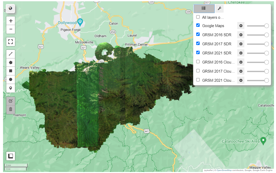
    Map.addLayer(image, visParams, layer_name)

# Center the map on the site
grsmCenter = ee.Geometry.Point([-83.5, 35.65]);
Map.centerObject(grsmCenter, 11);
Map

Adding GRSM 2016 Directional Reflectance
Adding GRSM 2017 Directional Reflectance
Adding GRSM 2021 Directional Reflectance

The function below extracts the weather quality band for each year of data in the image collection.

def yearly_weather_band(year):

    start_date = ee.Date.fromYMD(year, 1, 1) 
    end_date = start_date.advance(1, "year")
    
#     print('filtering image collection by date and site')
    aop_refl001 = refl001 \
        .filterDate(start_date, end_date) \
        .filterMetadata('NEON_SITE', 'equals', site).mosaic()
    
    # Extract Weather Quality Indicator band
    weather_quality_band = aop_refl001.select(['Weather_Quality_Indicator']);

    return weather_quality_band

Similarly, we will map this function over the list of years, and then add these weather quality images to the Map layer in a loop. For this we can define a color palette that will match AOP's weather stop-light color convention, where green means good weather (<10% cloud cover), yellow is OK (10-50% cloud cover), and red is bad (>50% cloud cover).

Map = geemap.Map()

weather_bands = years.map(yearly_weather_band)

# Define a palette for the weather - to match NEON AOP's weather color conventions (green-yellow-red)
gyrPalette = ['green', 'yellow', 'red']; # green: <10% cloud cover, yellow: 10-50% cloud cover, red: > 50% cloud cover

# parameters to display the weather bands (cloud conditions) with the green-yellow-red palette
weather_visParams = {'min': 1, 'max': 3, 'palette': gyrPalette, 'opacity': 0.3};

# loop through the layers and add them to the Map
for index in range(0, len(years.getInfo())):
    weather_band = ee.Image(weather_bands.get(index))
    layer_name = site + " " + str(years.getInfo()[index]) + " Cloud Cover Layer" 
    print('Adding ' + layer_name)
    Map.addLayer(weather_band, weather_visParams, layer_name, 1) # can change 1 to 0 if you don't want the layers to be selected "on" by default

Map.centerObject(grsmCenter, 11);
Map

Adding GRSM 2016 Cloud Cover Layer
Adding GRSM 2017 Cloud Cover Layer
Adding GRSM 2021 Cloud Cover Layer

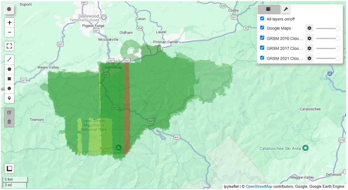
You can toggle on and off layers by selecting or deselecting each in the Layers window in the upper right corner.

Now let's add a full image collection (all years) for a different site onto the Map. For this example, we'll use the site Lyndon B. Johnson National Grassland (CLBJ), as there are 5 years of reflectance data ingested in GEE for that site. This is a nice example for displaying the time-lapse feature in the interactive map.

# Define the site code
site = 'CLBJ'

# Display the years of data available for the specified site:
print('\nReflectance data available in GEE for site',site,':')
print([year_site[0] for year_site in zip(refl001_years,refl001_sites) if site in year_site])

Reflectance data available in GEE for site CLBJ :
[2016, 2017, 2019, 2021]

Map = geemap.Map()

# Filter the refl001 and refl002 image collections at the selected site from all available years
site_refl001 = refl001.filterMetadata('NEON_SITE', 'equals', site);
site_refl002 = refl002.filterMetadata('NEON_SITE', 'equals', site);

# Read in only the data bands, all of which start with "B", eg. "B001"
site_refl001_data = site_refl001.select('B.*')
site_refl002_data = site_refl002.select('B.*')

# Read in the weather quality indicator band
site_refl001_weatherQA = site_refl001.select(['Weather_Quality_Indicator']);
site_refl002_weatherQA = site_refl002.select(['Weather_Quality_Indicator']);

# Set the visualization parameters so contrast is maximized, and display RGB bands (true-color image)
visParams = {'min':0,'max':1200,'gamma':0.9,'bands':['B053','B035','B019']};

# Add the site image collection as a layer to the Map
Map.addLayer(site_refl001_data, visParams, site + ' Refl 001');
Map.addLayer(site_refl002_data, visParams, site + ' Refl 002');

# Add the weather quality indicator (WQI) layer as well, for context
Map.addLayer(site_refl001_weatherQA, weather_visParams, site + ' Refl 001 WQI',0)
Map.addLayer(site_refl002_weatherQA, weather_visParams, site + ' Refl 002 WQI',0)

# Center the map on the site reflectance imaage
Map.centerObject(site_refl001, 12);
Map

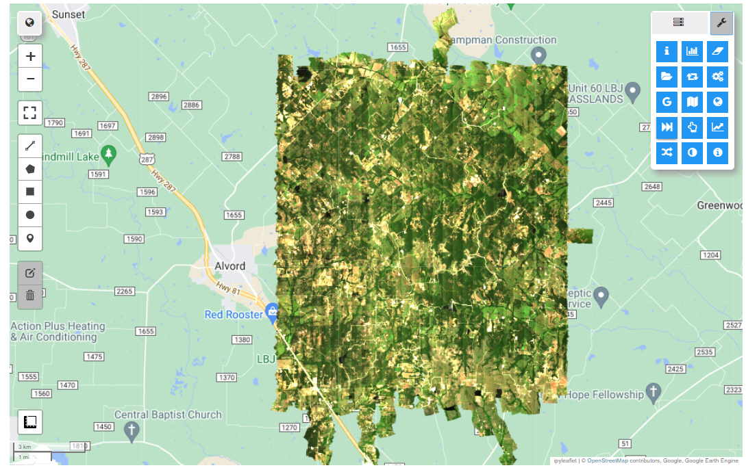
You should now see the Map panel populated with the CLBJ Image Collection and the Weather Quality Band. On your own, explore some of the options by click on the icon in the upper right corner of the map. Some options of interest may be the Create timelapse (globe icon), Inspector (I icon), and GEE toolbox for cloud computing. You can open and close the Layers window and interactively explore the different layers.

Create a Time-Lapse GIF

Lastly, optionally, we can create a time-lapse gif of the site over all the collections. This part follows along code from the GeoPython 2021 workshop: .

from geemap import cartoee
import matplotlib.pyplot as plt

# Define width and height (in degrees)
w = 0.1
h = 0.1

region = [lon - w, lat - h, lon + w, lat + h]

fig = plt.figure(figsize=(10, 8))

# Use cartoee to get a map
ax = geemap.cartoee.get_map(image, region=region, vis_params=visParams)

# Add gridlines to the map at a specified interval
geemap.cartoee.add_gridlines(ax, interval=[0.05, 0.05], linestyle=":")

# Add scale bar
scale_bar_dict = {
    "length": 10,
    "xy": (0.1, 0.05),
    "linewidth": 3,
    "fontsize": 20,
    "color": "white",
    "unit": "km",
    "ha": "center",
    "va": "bottom",
}
cartoee.add_scale_bar_lite(ax, **scale_bar_dict)

ax.set_title(label='CLBJ', fontsize=15)

plt.show()

We can then apply these settings and create the timelaps using cartoee.get_image_collection_gif as follows. This will create a "timelapse" subfolder in the Downloads directory.

cartoee.get_image_collection_gif(
    ee_ic=siteSDR,
    out_dir=os.path.expanduser("~/Downloads/timelapse"),
    out_gif="clbj_gee_timelapse.gif",
    vis_params=visParams,
    region=region,
    fps=1,
    mp4=True,
    grid_interval=(0.05, 0.05),
    plot_title="CLBJ AOP SDR Time Lapse",
    date_format='YYYY-MM-dd',
    fig_size=(10, 8),
    dpi_plot=100,
    file_format="png",
    scale_bar_dict=scale_bar_dict,
)

Recap

In this lesson we covered how to read in AOP Surface Directional Reflectance (SDR) datasets into GEE using Python with the packages ee and geemap. You learned how to write functions that mask out any data collected in >10% cloud cover conditions. You also got a chance to explore the interactive mapping tools that are made available as part of geemap. We encourage you to start writing functions and Python code on your own to expand upon these examples!