Tutorial
Cleaning and Gap-Filling NEON Aquatic Instrument Data
Last Updated: Mar 31, 2025
This tutorial covers some basic strategies for cleaning National Ecological Observatory Network (NEON) Level 1 Aquatic Instrument System (AIS) data prior to use.
Objectives
After completing this activity, you will be able to:
- Use the quality flags and issue logs to identify and remove suspect data.
- Use the calibration records to correct for drift and shifts.
- Fill small gaps in the data record.
Things You'll Need To Complete This Tutorial
To complete this tutorial you will need R (version >4.1) and, preferably, RStudio loaded on your computer.
Install R Packages
- neonUtilities: Access, download and compile NEON data
- ggplot2: Plotting functions
- zoo: Functions for working with time series
- kableExtra: Tool for building tables
These packages are on CRAN and can be installed by
install.packages().
Additional Resources
Download and Visually Inspect the Data
Before we get started, we need to install (if not already done) and load the required R packages.
# Install the required package if you have not yet.

install.packages("neonUtilities")

install.packages("ggplot2")

install.packages("zoo")

install.packages("kableExtra")


# Load required packages

library(neonUtilities)

library(ggplot2)

library(zoo)

library(kableExtra)
Part 1. Water Quality
For the first part of this tutorial we will use two months (2024-04 to 2024-05) of Water Quality (DP1.20288.001) from Walker Branch, Tennessee (WALK).
Download and Visually Inspect the Data
We will first use the loadByProduct() function in the neonUtilities package
to download data from the NEON API. For more information about using
neonUtilities to download data, use the tutorial linked in the Additional
Resources section above. Be sure to download the expanded data package so that
individual quality flags and Calibration Records are included.
waq <- neonUtilities::loadByProduct(dpID="DP1.20288.001", site="WALK",
                     startdate="2024-04", enddate="2024-05",
                     package="expanded", release="current",
                     include.provisional=T,
                     check.size=F)

list2env(waq,.GlobalEnv)
For wadeable stream sites, Water Quality is measured at multiple locations. For this tutorial, we'll only be using the downstream dataset. We can subset the data using the horizontalPosition variable. For more information about using the horizontalPosition and verticalPosition, use the tutorial linked in the Additional Resources section above.
waq_down<-waq_instantaneous[(waq_instantaneous$horizontalPosition==102),]
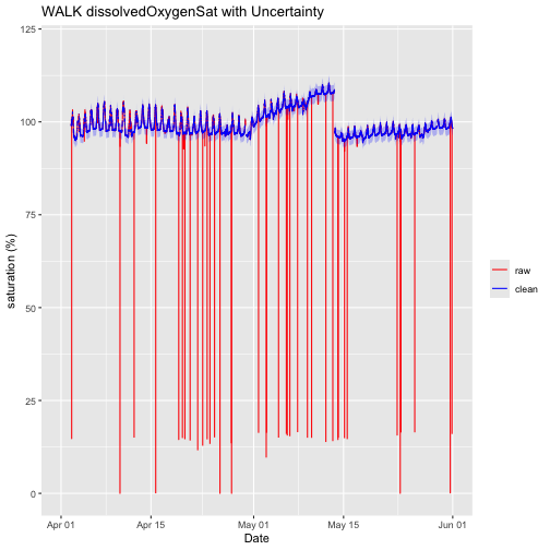
Water Quality includes multiple parameters. For this tutorial, we'll focus on local dissolved oxygen saturation at the downstream location. We'll first plot the raw data just to get a feel for what it looks like. We can also include uncertainty bands.
doPlotRaw <- ggplot() +
	geom_line(data = waq_down,aes(startDateTime, localDissolvedOxygenSat, colour="raw"),na.rm=TRUE) +
  geom_ribbon(data=waq_down,aes(x=startDateTime,
                  ymin = (localDissolvedOxygenSat - localDOSatExpUncert),
                  ymax = (localDissolvedOxygenSat + localDOSatExpUncert)),
                  alpha = 0.3, fill = "red") +
  scale_colour_manual("",breaks=c("raw"),values=c("red")) +
	ylim(0, 120) + ylab("saturation (%)") + xlab("Date")+ ggtitle("WALK dissolvedOxygenSat with Uncertainty")

doPlotRaw

Reviewing Issue Log
Each NEON data product comes with an Issue Log documenting major problems and any changes that have been made to the data product. We'll first filter the Issue Log for any records pertaining to this site and date range.
issueLog_20288<-issueLog_20288[(grepl(unique(waq_instantaneous$siteID),
                                      issueLog_20288$locationAffected))]

issueLog_20288<-issueLog_20288[!((issueLog_20288$dateRangeStart>
                                    max(waq_instantaneous$startDateTime))
              |(issueLog_20288$dateRangeEnd<
                  min(waq_instantaneous$startDateTime))),]

issueLog_20288 %>%
  kbl() %>%
    kable_styling()
| id | parentIssueID | issueDate | resolvedDate | dateRangeStart | dateRangeEnd | locationAffected | issue | resolution |
|---|---|---|---|---|---|---|---|---|
| 89108 | 89104 | 2024-06-17T00:00:00Z | 2024-06-17T00:00:00Z | 2024-04-29T00:00:00Z | 2024-05-13T00:00:00Z | WALK (101.001; 102.001) | Dissolved Oxygen sensor is drifting. | Sensor was cleaned and recalibrated if necessary. The cleaning and calibration records can be used to post-correct for this drift. |
We can see that there is an Issue Log entry indicating that the downstream dissolved oxygen sensor drifted, and that the Cleaning and Calibration records can be used to post-correct the data. That is something we should do in a subsequent step.
Filtering using NEON Quality Flags
NEON uses both automated and manual quality flags to identify data that is potentially suspect. Because we downloaded the expanded data package, we can filter using individual quality flags (e.x. range, step, spike) in addition to the final quality flag which combines the individual quality flags. For more information about interpreting quality flags, use the tutorial linked in the Additional Resources section above.
Flagged values are not removed from Level 1 NEON Instrument Systems data. It is the responsibility of the user to review quality flagged data to understand why it was flagged, and make their own determination whether they feel comfortable using it. For the tutorial we'll assume that we reviewed all the flagged data and determined any data with a final quality flag should be removed. We'll create a new column in the data table for the cleaned values. We’ll initially populate it with the raw values as a starting point, and then set any with a final quality flag to NA.
waq_down$cleanDissolvedOxygenSat<-waq_down$localDissolvedOxygenSat

waq_down$cleanDissolvedOxygenSat[waq_down$localDOSatFinalQF == 1] <- NA
Customized Data Filtering
Because the NEON automated quality flagging algorithm is not perfect, there may be times where additional filtering of potentially suspect data may be warranted (as well as times where potentially usable data has been erroneously quality flagged).
As an example of how to further filter data, we can create a customized step test where any pair of sequential points with a difference greater than a specified threshold will be set to NA. We could also make this test apply to only certain time periods.
stepStart <- as.POSIXct("2024-04-01 00:00:00",tz="GMT")

stepEnd <- as.POSIXct("2024-06-01 00:00:00",tz="GMT")

maxStep <- 0.1

for(i in 2:nrow(waq_down)){if((waq_down$startDateTime[i]>stepStart)&
                              (waq_down$endDateTime[i]<stepEnd)){
  if((!is.na(waq_down$localDissolvedOxygenSat[i]))&
     (!is.na(waq_down$localDissolvedOxygenSat[i-1]))){
    if(abs(waq_down$localDissolvedOxygenSat[i]-
       waq_down$localDissolvedOxygenSat[i-1])>maxStep){
          waq_down$cleanDissolvedOxygenSat[i] <- NA
          waq_down$cleanDissolvedOxygenSat[i-1] <- NA
      }}}}
Alternatively, we could create a customized range test where any values outside a specified minimum and maximum are set to NA. For example, Dissolved Oxygen saturation in most healthy streams is usually around 100%, and values far outside this range might be erroneous.
rangeStart <- as.POSIXct("2024-04-01 00:00:00",tz="GMT")

rangeEnd <- as.POSIXct("2024-06-01 00:00:00",tz="GMT")

minRange <- 80

maxRange <- 120

for(i in 1:nrow(waq_down)){
  if((waq_down$startDateTime[i]>rangeStart)&(waq_down$endDateTime[i]<rangeEnd)){
    if((!is.na(waq_down$localDissolvedOxygenSat[i]))){
      if((waq_down$localDissolvedOxygenSat[i]<minRange)|
         (waq_down$localDissolvedOxygenSat[i]>maxRange)){
            waq_down$cleanDissolvedOxygenSat[i] <- NA
            }}}}
Now that we have removed the quality flagged values, let's re-plot the data. We'll use red for the raw data and blue for the clean data.
doPlotQF <- ggplot() +
	geom_line(data = waq_down,aes(startDateTime, localDissolvedOxygenSat, colour="raw"),na.rm=TRUE) +
  geom_line(data = waq_down,aes(startDateTime, cleanDissolvedOxygenSat, colour="clean"),na.rm=TRUE) +
  geom_ribbon(data=waq_down,aes(x=startDateTime,
                  ymin = (cleanDissolvedOxygenSat - localDOSatExpUncert),
                  ymax = (cleanDissolvedOxygenSat + localDOSatExpUncert)),
                  alpha = 0.3, fill = "blue") +
  scale_colour_manual("",breaks=c("raw","clean"),values=c("red","blue")) +
	ylim(0, 120) + ylab("saturation (%)") + xlab("Date")+ ggtitle("WALK dissolvedOxygenSat with Uncertainty")

doPlotQF
Drift Correction using Cleaning and Calibration Records
The drift and calibration correction methods outlined here are based off the Guidelines and Procedures for Continuous Water-Quality Monitoring used by the United States Geological Survey and found in Techniques and Methods 1-D3
We'll try and fix the drifting downstream sensor noted in the Issue Log using the Cleaning and Calibration records. The records for Water Quality include multiple sensors. We'll first filter the records to just those related to dissolved oxygen.
doCleanCal<-ais_multisondeCleanCal[,c("startDate","s1PreCleaningDO",
                          "s2PreCleaningDO","s1PostCleaningDO",
                          "s2PostCleaningDO","s1DOCalSuccessful",
                          "s2DOCalSuccessful","s1BucketDO",
                          "s2BucketDO")]

doCleanCal %>%
  kbl() %>%
    kable_styling()
| startDate | s1PreCleaningDO | s2PreCleaningDO | s1PostCleaningDO | s2PostCleaningDO | s1DOCalSuccessful | s2DOCalSuccessful | s1BucketDO | s2BucketDO |
|---|---|---|---|---|---|---|---|---|
| 2024-04-03 16:00:00 | 103.2 | 98.5 | 100.6 | 99.2 | Y | Y | 94.7 | 95.1 |
| 2024-04-16 16:00:00 | 94.8 | 95.1 | 95.2 | 95.9 | NA | NA | NA | NA |
| 2024-04-29 16:00:00 | 94.5 | 94.4 | 96.4 | 95.4 | Y | Y | 100.0 | 99.8 |
| 2024-05-01 16:00:00 | NA | NA | NA | NA | NA | NA | NA | NA |
| 2024-05-13 16:00:00 | 95.5 | 106.1 | 94.8 | 95.5 | NA | NA | NA | NA |
| 2024-05-29 16:00:00 | 94.0 | 96.1 | 95.2 | 97.9 | NA | NA | NA | NA |
We can see in the Cleaning and Calibration records that on 2024-05-13 the downstream (S2) sensor was reading 106.1% pre-cleaning, but only 95.5% post-cleaning. Alternatively, we could look at the actual data, where the last measurement prior to cleaning was was 108.7% and the first measurement after cleaning was 97.6%. These pairs of measurements are often not exactly the same because of the process of physically removing the sensor from the stream, the concentration in the stream may be changing during the cleaning, and the uncertainty associated with the measurement itself.
If we assume that the rate of drift was constant, we can subtract a linearly increasing offset going back to the previous cleaning and calibration on 2024-04-29. Alternatively, we could set a different start and/or end date if we believe the drift only occurred during part of a cleaning and calibration interval.
driftStart <- as.POSIXct("2024-04-29 17:00:00",tz="GMT")

driftEnd <- as.POSIXct("2024-05-13 15:00:00",tz="GMT")

drift <- 106.1-95.5

  for(i in 1:nrow(waq_down)){
    if(waq_down$startDateTime[i]>driftStart&
       waq_down$startDateTime[i]<driftEnd){
        waq_down$cleanDissolvedOxygenSat[i] <-
          waq_down$cleanDissolvedOxygenSat[i]-
          (drift*(as.numeric(difftime(waq_down$startDateTime[i],
                          driftStart,units="secs"))/
                    as.numeric(difftime(driftEnd,
                          driftStart,units="secs"))))
        }}
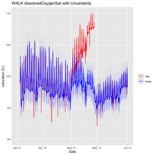
Let's re-plot the data and see what these adjustments have done.
doPlotDrift <- ggplot() +
	geom_line(data = waq_down,aes(startDateTime, localDissolvedOxygenSat, colour="raw"),na.rm=TRUE) +
  geom_line(data = waq_down,aes(startDateTime, cleanDissolvedOxygenSat, colour="clean"),na.rm=TRUE) +
  geom_ribbon(data=waq_down,aes(x=startDateTime,
                  ymin = (cleanDissolvedOxygenSat - localDOSatExpUncert),
                  ymax = (cleanDissolvedOxygenSat + localDOSatExpUncert)),
                  alpha = 0.3, fill = "blue") +
  scale_colour_manual("",breaks=c("raw","clean"),values=c("red","blue")) +
	ylim(90, 110) + ylab("saturation (%)") + xlab("Date")+ ggtitle("WALK dissolvedOxygenSat with Uncertainty")

doPlotDrift

Basic Gap Filling
Level 1 NEON Instrument Systems data is not gap filled. Data gaps may result either from periods when data was not collected, or when erroneous data was removed during the cleaning process.
Many analyses require continuous data sets with no gaps. Other analyses (e.g. calculation of long term averages) require that gaps be randomly distributed, which often may not be the case.
Because the gaps in our example here are relatively short (on the order of minutes to hours), it is probably safe to use simple linear interpolation. We can do this using the na.approx function in the zoo package.
waq_down$cleanDissolvedOxygenSat<-
  zoo::na.approx(waq_down$cleanDissolvedOxygenSat,maxgap=300)
Let's re-plot the data and see what the gap filled data look like.
doPlotFilled <- ggplot() +
	geom_line(data = waq_down,aes(startDateTime, localDissolvedOxygenSat, colour="raw"),na.rm=TRUE) +
  geom_line(data = waq_down,aes(startDateTime, cleanDissolvedOxygenSat, colour="clean"),na.rm=TRUE) +
  geom_ribbon(data=waq_down,aes(x=startDateTime,
                  ymin = (cleanDissolvedOxygenSat - localDOSatExpUncert),
                  ymax = (cleanDissolvedOxygenSat + localDOSatExpUncert)),
                  alpha = 0.3, fill = "blue") +
  scale_colour_manual("",breaks=c("raw","clean"),values=c("red","blue")) +
	ylim(90, 110) + ylab("saturation (%)") + xlab("Date")+ ggtitle("WALK dissolvedOxygenSat with Uncertainty")

doPlotFilled
Longer gaps require more sophisticated gap filling methods. At NEON sites, some parameters are measured by multiple sensors at nearby locations. Depending on the degree of spatial heterogeneity, data from one location could be used to gap fill at another location.
A more complicated approach could be to use process-based modeling. For example, water temperature is likely related to air temperature or dissolved oxygen is likely related to solar insolation via photosynthesis. However, these cross-variable relationships are often the very thing we are trying to analyze. Carefully consider your analytical approach and hypotheses before deciding whether to fill gaps, and which methods to use. Also note that gap filling adds additional uncertainty.
Part 2. Nitrate in Surface Water
For the second part of this tutorial we will use two months (2024-01 to 2024-02) of Nitrate in surface water (DP1.20033.001) from Walker Branch, Tennessee (WALK).
Download and Visually Inspect the Data
We will first download the expanded package for Nitrate in surface water using
the neonUtilities package.
nsw <- neonUtilities::loadByProduct(dpID="DP1.20033.001", site="WALK",
                     startdate="2024-01", enddate="2024-02",
                     package="expanded", release="current",
                     include.provisional=T,
                     check.size=F)

list2env(nsw,.GlobalEnv)
Let's then check how many locations are present using horizontalPosition.
print(unique(NSW_15_minute$horizontalPosition))

## [1] "102"
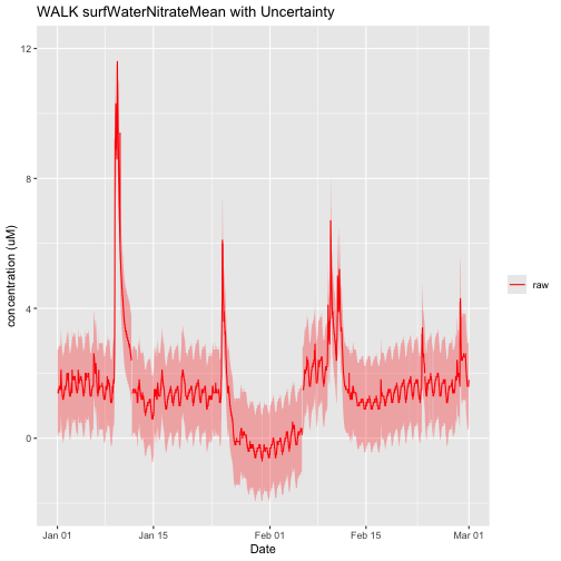
There should only be one horizontalPosition present, because NEON only measures Nitrate in surface water at the downstream location for wadeable stream sites. Therefore, we do not need to subset this dataset like we did for Water quality. We can now plot the data, including uncertainty bands.
nswPlotRaw <- ggplot() +
	geom_line(data = NSW_15_minute,aes(startDateTime, surfWaterNitrateMean, colour="raw"),na.rm=TRUE) +
  geom_ribbon(data=NSW_15_minute,aes(x=startDateTime,
                  ymin = (surfWaterNitrateMean - surfWaterNitrateExpUncert),
                  ymax = (surfWaterNitrateMean + surfWaterNitrateExpUncert)),
                  alpha = 0.3, fill = "red") +
  scale_colour_manual("",breaks=c("raw"),values=c("red")) +
	ylim(-2, 12) + ylab("concentration (uM)") + xlab("Date")+ ggtitle("WALK surfWaterNitrateMean with Uncertainty")

nswPlotRaw
Review Issue Log and Remove Quality Flagged data.
It looks like there is are some small shifts in the data on 2024-01-11 and 2024-02-05. Let's review the issue log to see if it has any more information about this shift. Just like we did for Water quality, we'll filter the log for records pertaining to this site and date range.
issueLog_20033<-issueLog_20033[(grepl(unique(NSW_15_minute$siteID),
                                      issueLog_20033$locationAffected))]

issueLog_20033<-issueLog_20033[!((issueLog_20033$dateRangeStart>
                                    max(NSW_15_minute$startDateTime))
              |(issueLog_20033$dateRangeEnd<
                  min(NSW_15_minute$startDateTime))),]

issueLog_20033 %>%
  kbl() %>%
    kable_styling()
| id | parentIssueID | issueDate | resolvedDate | dateRangeStart | dateRangeEnd | locationAffected | issue | resolution |
|---|---|---|---|---|---|---|---|---|
We can see that there are no Issue Log entries for Nitrate in surface water at Walker Branch during this date range.
Next, let's remove any quality flagged measurements.
NSW_15_minute$cleanSurfWaterNitrate<-NSW_15_minute$surfWaterNitrateMean

NSW_15_minute$cleanSurfWaterNitrate[NSW_15_minute$finalQF == 1] <- NA
We can then re-plot the cleaned data
nswPlotQF <- ggplot() +
	geom_line(data = NSW_15_minute,aes(startDateTime, surfWaterNitrateMean, colour="raw"),na.rm=TRUE) +
  geom_line(data = NSW_15_minute,aes(startDateTime, cleanSurfWaterNitrate, colour="clean"),na.rm=TRUE) +
  geom_ribbon(data=NSW_15_minute,aes(x=startDateTime,
                  ymin = (cleanSurfWaterNitrate - surfWaterNitrateExpUncert),
                  ymax = (cleanSurfWaterNitrate + surfWaterNitrateExpUncert)),
                  alpha = 0.3, fill = "blue") +
  scale_colour_manual("",breaks=c("raw","clean"),values=c("red","blue")) +
	ylim(-2, 12) + ylab("concentration (uM)") + xlab("Date")+ ggtitle("WALK surfWaterNitrateMean with Uncertainty")

nswPlotQF
It looks like the shifts in the data also were not quality flagged. These shifts were likely not included in the Issue Log or quality flagged because they are still within the uncertainty of the sensor.
Correcting Calibration Shifts
Shifts caused by poor calibration can often be corrected using the pre- and post-calibration measurements found in the Cleaning and Calibration Records, similar to how we corrected for drift in the Water Quality data.
nswCleanCal<-ais_sunaCleanAndCal[,c("collectDate","preCleanNitrateBlankConc",
                          "postCleanNitrateBlankConc","postCalNitrateBlankConc")]

nswCleanCal %>%
  kbl() %>%
    kable_styling()
| collectDate | preCleanNitrateBlankConc | postCleanNitrateBlankConc | postCalNitrateBlankConc |
|---|---|---|---|
| 2024-01-11 17:00:00 | -0.34 | -0.62 | 0.85 |
| 2024-02-05 17:00:00 | -0.65 | -1.83 | -1.72 |
From the Cleaning and Calibration Records, we can see that calibrations were indeed performed on the dates of the shift. However, we can also see that on 2024-01-11, the post-calibration measurement of 0.85 (made in deionized water) was higher than the pre-cleaning and calibration measurement of -0.34, yet the data following that calibration shift downward. Conversely, on 2024-02-05 the post-calibration measurement of -1.72 was less than the pre-cleaning and calibration measurement of -0.65, yet the data following that calibration shift upward. In actuality, all of the differences (both between pre- versus post- calibrations and the shifts in the actual data) are within the uncertainty of the sensor.
Sometimes the data cleaning process must rely on professional judgement. While it is unclear from the Cleaning and Calibration Records which data should be shifted up or down, the negative values during the period from 2024-01-11 to 2024-02-05 are a good indication that this period should be shifted upwards. We can do this by applying a manual shift correction to this time period.
A shift correction can take multiple forms. We can either add/subtract a value for an issue with an offset (intercept), and/or multiplying by a value for an issue with the gain (slope). For this example, let's apply a constant offset of +1.1 and leave the gain as 1.
shiftStart <- as.POSIXct("2024-01-11 20:00:00",tz="GMT")

shiftEnd <- as.POSIXct("2024-02-05 16:00:00",tz="GMT")

offset <- 1.1

gain <- 1

  for(i in 1:nrow(NSW_15_minute)){
    if(NSW_15_minute$startDateTime[i]>shiftStart&NSW_15_minute$startDateTime[i]<shiftEnd){
      NSW_15_minute$cleanSurfWaterNitrate[i] <-
        NSW_15_minute$cleanSurfWaterNitrate[i]*gain+offset}}
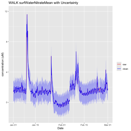
We can then re-plot the shifted data.
nswPlotShift <- ggplot() +
	geom_line(data = NSW_15_minute,aes(startDateTime, surfWaterNitrateMean, colour="raw"),na.rm=TRUE) +
  geom_line(data = NSW_15_minute,aes(startDateTime, cleanSurfWaterNitrate, colour="clean"),na.rm=TRUE) +
  geom_ribbon(data=NSW_15_minute,aes(x=startDateTime,
                  ymin = (cleanSurfWaterNitrate - surfWaterNitrateExpUncert),
                  ymax = (cleanSurfWaterNitrate + surfWaterNitrateExpUncert)),
                  alpha = 0.3, fill = "blue") +
  scale_colour_manual("",breaks=c("raw","clean"),values=c("red","blue")) +
	ylim(-2, 12) + ylab("concentration (uM)") + xlab("Date")+ ggtitle("WALK surfWaterNitrateMean with Uncertainty")

nswPlotShift
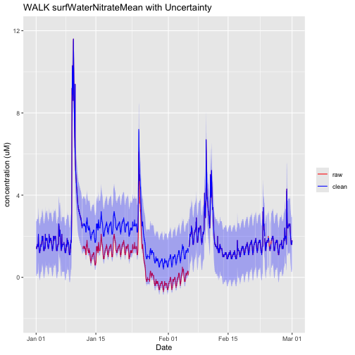
We can see that the shifted data now align more closely with the preceding and succeeding time periods. Note that the shift is still within the uncertainty range.
Conclusions
Most NEON Level 1 Data Products require some level of cleaning and/or gap filling as part of the analytical process. NEON provides automated and manual quality flags, Issue Logs and Calibration Records to aid users in this process. Users with questions are encouraged to reach out to NEON.
Data cleaning will almost always include some amount of subjective judgement. For data being used in publications, NEON recommends that for transparency and reproducibility, the process for cleaning the data be documented in the methods, and that the code used and the cleaned data set be archived in a publicly accessible repository.