Tutorial
Create a Canopy Height Model from Lidar-derived rasters in R
Last Updated: Feb 6, 2024
A common analysis using lidar data are to derive top of the canopy height values from the lidar data. These values are often used to track changes in forest structure over time, to calculate biomass, and even leaf area index (LAI). Let's dive into the basics of working with raster formatted lidar data in R!
Learning Objectives
After completing this tutorial, you will be able to:
- Work with digital terrain model (DTM) & digital surface model (DSM) raster files.
- Create a canopy height model (CHM) raster from DTM & DSM rasters.
Things You’ll Need To Complete This Tutorial
You will need the most current version of R and, preferably, RStudio loaded
on your computer to complete this tutorial.
Install R Packages
-
terra:
install.packages("terra") -
neonUtilities:
install.packages("neonUtilities")
More on Packages in R - Adapted from Software Carpentry.
Download Data
Lidar elevation raster data are downloaded using the R neonUtilities::byTileAOP function in the script.
These remote sensing data files provide information on the vegetation at the National Ecological Observatory Network's San Joaquin Experimental Range and Soaproot Saddle field sites. The entire datasets can be accessed from the .
This tutorial is designed for you to set your working directory to the directory created by unzipping this file.
Set Working Directory: This lesson will walk you through setting the working directory before downloading the datasets from neonUtilities.
An overview of setting the working directory in R can be found here.
R Script & Challenge Code: NEON data lessons often contain challenges to reinforce skills. If available, the code for challenge solutions is found in the downloadable R script of the entire lesson, available in the footer of each lesson page.
Recommended Reading
What is a CHM, DSM and DTM? AGŐćČË°ŮĽŇŔֹٷ˝ÍřŐľ Gridded, Raster LiDAR DataCreate a lidar-derived Canopy Height Model (CHM)
The National Ecological Observatory Network (NEON) will provide lidar-derived data products as one of its many free ecological data products. These products will come in the format, which is a .tif raster format that is spatially located on the earth.
In this tutorial, we create a Canopy Height Model. The Canopy Height Model (CHM), represents the heights of the trees on the ground. We can derive the CHM by subtracting the ground elevation from the elevation of the top of the surface (or the tops of the trees).
We will use the terra R package to work with the the lidar-derived Digital
Surface Model (DSM) and the Digital Terrain Model (DTM).
# Load needed packages

library(terra)

library(neonUtilities)
Set the working directory so you know where to download data.
wd="~/data/" #This will depend on your local environment

setwd(wd)
We can use the neonUtilities function byTileAOP to download a single DTM and DSM tile at SJER. Both the DTM and DSM are delivered under the data product.
You can run help(byTileAOP) to see more details on what the various inputs are. For this exercise, we'll specify the UTM Easting and Northing to be (257500, 4112500), which will download the tile with the lower left corner (257000,4112000). By default, the function will check the size total size of the download and ask you whether you wish to proceed (y/n). You can set check.size=FALSE if you want to download without a prompt. This example will not be very large (~8MB), since it is only downloading two single-band rasters (plus some associated metadata).
byTileAOP(dpID='DP3.30024.001',

          site='SJER',

          year='2021',

          easting=257500,

          northing=4112500,

          check.size=TRUE, # set to FALSE if you don't want to enter y/n

          savepath = wd)
This file will be downloaded into a nested subdirectory under the ~/data folder, inside a folder named DP3.30024.001 (the Data Product ID). The files should show up in these locations: ~/data/DP3.30024.001/neon-aop-products/2021/FullSite/D17/2021_SJER_5/L3/DiscreteLidar/DSMGtif/NEON_D17_SJER_DP3_257000_4112000_DSM.tif and ~/data/DP3.30024.001/neon-aop-products/2021/FullSite/D17/2021_SJER_5/L3/DiscreteLidar/DTMGtif/NEON_D17_SJER_DP3_257000_4112000_DTM.tif.
Now we can read in the files. You can move the files to a different location (eg. shorten the path), but make sure to change the path that points to the file accordingly.
# Define the DSM and DTM file names, including the full path

dsm_file <- paste0(wd,"DP3.30024.001/neon-aop-products/2021/FullSite/D17/2021_SJER_5/L3/DiscreteLidar/DSMGtif/NEON_D17_SJER_DP3_257000_4112000_DSM.tif")

dtm_file <- paste0(wd,"DP3.30024.001/neon-aop-products/2021/FullSite/D17/2021_SJER_5/L3/DiscreteLidar/DTMGtif/NEON_D17_SJER_DP3_257000_4112000_DTM.tif")
First, we will read in the Digital Surface Model (DSM). The DSM represents the elevation of the top of the objects on the ground (trees, buildings, etc).
# assign raster to object

dsm <- rast(dsm_file)


# view info about the raster.

dsm

## class       : SpatRaster
## dimensions  : 1000, 1000, 1  (nrow, ncol, nlyr)
## resolution  : 1, 1  (x, y)
## extent      : 257000, 258000, 4112000, 4113000  (xmin, xmax, ymin, ymax)
## coord. ref. : WGS 84 / UTM zone 11N (EPSG:32611)
## source      : NEON_D17_SJER_DP3_257000_4112000_DSM.tif
## name        : NEON_D17_SJER_DP3_257000_4112000_DSM

# plot the DSM

plot(dsm, main="Lidar Digital Surface Model \n SJER, California")
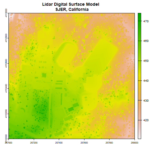
Note the resolution, extent, and coordinate reference system (CRS) of the raster. To do later steps, our DTM will need to be the same.
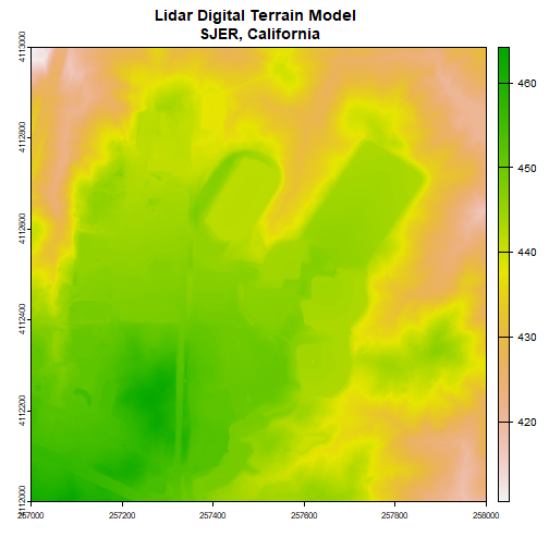
Next, we will import the Digital Terrain Model (DTM) for the same area. The DTM represents the ground (terrain) elevation.
# import the digital terrain model

dtm <- rast(dtm_file)


plot(dtm, main="Lidar Digital Terrain Model \n SJER, California")
With both of these rasters now loaded, we can create the Canopy Height Model (CHM). The CHM represents the difference between the DSM and the DTM or the height of all objects on the surface of the earth.
To do this we perform some basic raster math to calculate the CHM. You can perform the same raster math in a GIS program like .
When you do the math, make sure to subtract the DTM from the DSM or you'll get trees with negative heights!
# use raster math to create CHM

chm <- dsm - dtm


# view CHM attributes

chm

## class       : SpatRaster
## dimensions  : 1000, 1000, 1  (nrow, ncol, nlyr)
## resolution  : 1, 1  (x, y)
## extent      : 257000, 258000, 4112000, 4113000  (xmin, xmax, ymin, ymax)
## coord. ref. : WGS 84 / UTM zone 11N (EPSG:32611)
## source(s)   : memory
## varname     : NEON_D17_SJER_DP3_257000_4112000_DSM
## name        : NEON_D17_SJER_DP3_257000_4112000_DSM
## min value   :                                 0.00
## max value   :                                24.13

plot(chm, main="Lidar CHM - SJER, California")
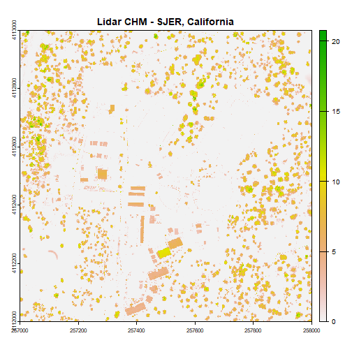
We've now created a CHM from our DSM and DTM. What do you notice about the canopy cover at this location in the San Joaquin Experimental Range?
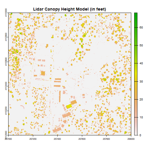
Challenge: Basic Raster Math
Convert the CHM from meters to feet and plot it.
We can write out the CHM as a GeoTiff using the writeRaster() function.
# write out the CHM in tiff format.

writeRaster(chm,paste0(wd,"CHM_SJER.tif"),"GTiff")
We've now successfully created a canopy height model using basic raster math -- in
R! We can bring the CHM_SJER.tif file into QGIS (or any GIS program) and look
at it.
Consider checking out the tutorial Compare tree height measured from the ground to a Lidar-based Canopy Height Model to compare a LiDAR-derived CHM with ground-based observations!