Tutorial
Data Activity: Visualize Precipitation Data in R to Better Understand the 2013 Colorado Floods
Last Updated: Apr 10, 2025
Several factors contributed to extreme flooding that occurred in Boulder, Colorado in 2013. In this data activity, we explore and visualize the data for precipitation (rainfall) data collected by the National Weather Service's Cooperative Observer Program. The tutorial is part of the Data Activities that can be used with the Quantifying The Drivers and Impacts of Natural Disturbance Events Teaching Module.
Learning Objectives
After completing this tutorial, you will be able to:
- Download precipitation data from .
- Plot precipitation data in R.
- Publish & share an interactive plot of the data using Plotly.
- Subset data by date (if completing Additional Resources code).
- Set a NoData Value to NA in R (if completing Additional Resources code).
Things You'll Need To Complete This Lesson
Please be sure you have the most current version of R and, preferably, RStudio to write your code.
R Libraries to Install:
-
ggplot2:
install.packages("ggplot2") -
plotly:
install.packages("plotly")
Data to Download
Part of this lesson is to access and download the data directly from NOAA's NCEI Database. If instead you would prefer to download the data as a single compressed file, it can be downloaded from the .
Set Working Directory This lesson assumes that you have set your working directory to the location of the downloaded and unzipped data subsets.
An overview of setting the working directory in R can be found here.
R Script & Challenge Code: NEON data lessons often contain challenges that reinforce learned skills. If available, the code for challenge solutions is found in the downloadable R script of the entire lesson, available in the footer of each lesson page.
Research Question
What were the patterns of precipitation leading up to the 2013 flooding events in Colorado?
Precipitation Data
The heavy precipitation (rain) that occurred in September 2013 caused much damage during the 2013 flood by, among other things, increasing stream discharge (flow). In this lesson we will download, explore, and visualize the precipitation data collected during this time to better understand this important flood driver.
Where can we get precipitation data?
The precipitation data are obtained through . There are numerous datasets that can be found and downloaded via the .
The precipitation data that we will use is from the .
"Through the National Weather Service (NWS) Cooperative Observer Program (COOP), more than 10,000 volunteers take daily weather observations at National Parks, seashores, mountaintops, and farms as well as in urban and suburban areas. COOP data usually consist of daily maximum and minimum temperatures, snowfall, and 24-hour precipitation totals." Quoted from NOAA's National Centers for Environmental Information
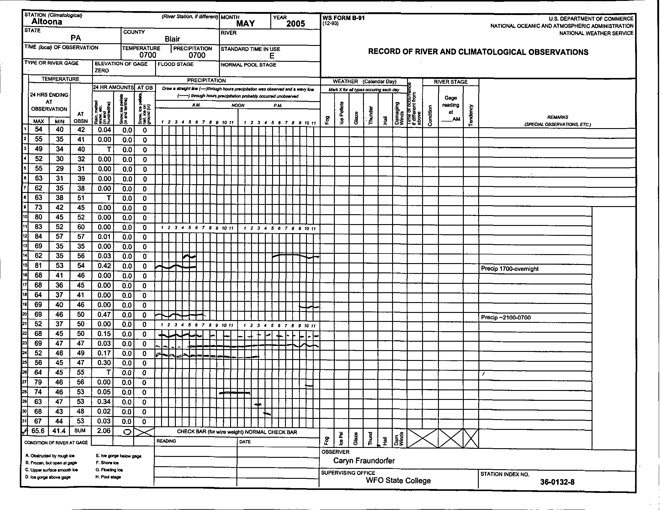
Data are collected at different stations, often on paper data sheets like the one below, and then entered into a central database where we can access that data and download it in the .csv (Comma Separated Values) format.
Obtain the Data
If you have not already opened the , do so now.
Note: If you are using the pre-compiled data subset that can be downloaded as a compressed file above, you should still read through this section to know where the data comes from before proceeding with the lesson.
Step 1: Search for the data
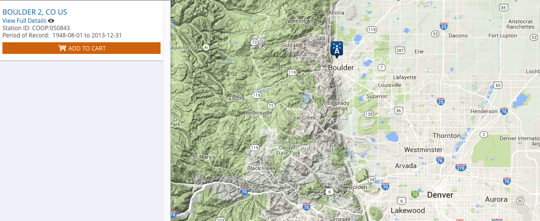
To obtain data we must first choose a location of interest. The COOP site Boulder 2 (Station ID:050843) is centrally located in Boulder, CO.
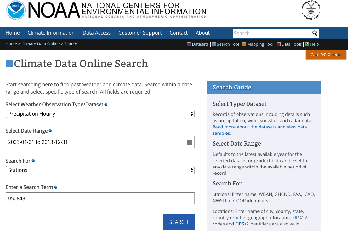
Then we must decide what type of data we want to download for that station. As shown in the image below, we selected:
- the desired date range (1 January 2003 to 31 December 2013),
- the type of dataset ("Precipitation Hourly"),
- the search type ("Stations") and
- the search term (e.g. the # for the station located in central Boulder, CO: 050843).
Once the data are entered and you select Search, you will be directed to a
new page with a map. You can find out more information about the data by selecting
View Full Details.
Notice that this dataset goes all the way back to 1 August 1948! However, we've
selected only a portion of this time frame.
Step 2: Request the data
Once you are sure this is the data that you want, you need to request it by
selecting Add to Cart. The data can then be downloaded as a .csv file
which we will use to conduct our analyses. Be sure to double check the date
range before downloading.
On the options page, we want to make sure we select:
- Station Name
- Geographic Location (this gives us longitude & latitude; optional)
- Include Data Flags (this gives us information if the data are problematic)
- Units (Standard)
- Precipitation (w/ HPCP automatically checked)
On the next page you must enter an email address for the dataset to be sent to.
Step 3: Get the data
As this is a small dataset, it won't take long for you to get an email telling
you the dataset is ready. Follow the link in the email to download your dataset.
You can also view documentation (metadata) for the data.
Each data subset is downloaded with a unique order number. The order number in
our example dataset is 805325. If you are using a dataset you've downloaded
yourself, make sure to substitute in your own order number in the code below.
To ensure that we remember what our data file is, we've added a descriptor to
the order number: 805325-precip_daily_2003-2013. You may wish to do the same.
Work with Precipitation Data
R Libraries
We will use ggplot2 to efficiently plot our data and plotly to create i
nteractive plots.
# load packages
library(ggplot2) # create efficient, professional plots
library(plotly) # create cool interactive plots

##
## Attaching package: 'plotly'

## The following object is masked from 'package:ggmap':
##
##     wind

## The following object is masked from 'package:ggplot2':
##
##     last_plot

## The following object is masked from 'package:stats':
##
##     filter

## The following object is masked from 'package:graphics':
##
##     layout

# set your working directory to ensure R can find the file we wish to import
# and where we want to save our files. Be sure to move the download into
# your working direectory!
wd <- "~/Git/data/" # This will depend on your local environment
setwd(wd)
Import Precipitation Data
We will use the 805325-Preciptation_daily_2003-2013.csv file
in this analysis. This dataset is the daily precipitation date from the COOP
station 050843 in Boulder, CO for 1 January 2003 through 31 December 2013.
Since the data format is a .csv, we can use read.csv to import the data. After
we import the data, we can take a look at the first few lines using head(),
which defaults to the first 6 rows, of the data.frame. Finally, we can explore
the R object structure.
# import precip data into R data.frame by
# defining the file name to be opened

precip.boulder <- read.csv(paste0(wd,"disturb-events-co13/precip/805325-precip_daily_2003-2013.csv"), stringsAsFactors = FALSE, header = TRUE )

# view first 6 lines of the data
head(precip.boulder)

##       STATION    STATION_NAME ELEVATION LATITUDE LONGITUDE
## 1 COOP:050843 BOULDER 2 CO US    1650.5 40.03389 -105.2811
## 2 COOP:050843 BOULDER 2 CO US    1650.5 40.03389 -105.2811
## 3 COOP:050843 BOULDER 2 CO US    1650.5 40.03389 -105.2811
## 4 COOP:050843 BOULDER 2 CO US    1650.5 40.03389 -105.2811
## 5 COOP:050843 BOULDER 2 CO US    1650.5 40.03389 -105.2811
## 6 COOP:050843 BOULDER 2 CO US    1650.5 40.03389 -105.2811
##             DATE HPCP Measurement.Flag Quality.Flag
## 1 20030101 01:00  0.0                g
## 2 20030201 01:00  0.0                g
## 3 20030202 19:00  0.2
## 4 20030202 22:00  0.1
## 5 20030203 02:00  0.1
## 6 20030205 02:00  0.1

# view structure of data
str(precip.boulder)

## 'data.frame':	1840 obs. of  9 variables:
##  $ STATION         : chr  "COOP:050843" "COOP:050843" "COOP:050843" "COOP:050843" ...
##  $ STATION_NAME    : chr  "BOULDER 2 CO US" "BOULDER 2 CO US" "BOULDER 2 CO US" "BOULDER 2 CO US" ...
##  $ ELEVATION       : num  1650 1650 1650 1650 1650 ...
##  $ LATITUDE        : num  40 40 40 40 40 ...
##  $ LONGITUDE       : num  -105 -105 -105 -105 -105 ...
##  $ DATE            : chr  "20030101 01:00" "20030201 01:00" "20030202 19:00" "20030202 22:00" ...
##  $ HPCP            : num  0 0 0.2 0.1 0.1 ...
##  $ Measurement.Flag: chr  "g" "g" " " " " ...
##  $ Quality.Flag    : chr  " " " " " " " " ...
AGŐćČË°ŮĽŇŔֹٷ˝ÍřŐľ the Data
Viewing the structure of these data, we can see that different types of data are included in this file.
- STATION and STATION_NAME: Identification of the COOP station.
- ELEVATION, LATITUDE and LONGITUDE: The spatial location of the station.
-
DATE: Gives the date in the format: YYYYMMDD HH:MM. Notice that DATE is
currently class
chr, meaning the data are interpreted as a character class and not as a date. -
HPCP: The total precipitation given in inches
(since we selected
Standardfor the units), recorded for the hour ending at the time specified by DATE. Importantly, the metadata (see below) notes that the value 999.99 indicates missing data. Also important, hours with no precipitation are not recorded. - Measurement Flag: Indicates if there are any abnormalities with the measurement of the data. Definitions of each flag can be found in Table 2 of the documentation.
- Quality Flag: Indicates if there are any potential quality problems with the data. Definitions of each flag can be found in Table 3 of the documentation.
Additional information about the data, known as metadata, is available in the
PRECIP_HLY_documentation.pdf file that can be downloaded along with the data.
(Note, as of Sept. 2016, there is a mismatch in the data downloaded and the
documentation. The differences are in the units and missing data value:
inches/999.99 (standard) or millimeters/25399.75 (metric)).
Clean the Data
Before we can start plotting and working with the data we always need to check several important factors:
- data class: is R interpreting the data the way we expect it. The function
str()is an important tools for this. - NoData Values: We need to know if our data contains a specific value that means "data are missing" and if this value has been assigned to NA in R.
Convert Date-Time
As we've noted, the date field is in a character class. We can convert it to a date/time
class that will allow R to correctly interpret the data and allow us to easily
plot the data. We can convert it to a date/time class using as.POSIXct().
# convert to date/time and retain as a new field
precip.boulder$DateTime <- as.POSIXct(precip.boulder$DATE,
                                  format="%Y%m%d %H:%M")
                                  # date in the format: YearMonthDay Hour:Minute

# double check structure
str(precip.boulder$DateTime)

##  POSIXct[1:1840], format: "2003-01-01 01:00:00" "2003-02-01 01:00:00" ...
- For more information on date/time classes, see the NEON tutorial Dealing With Dates & Times in R - as.Date, POSIXct, POSIXlt.
NoData Values
We've also learned that missing values, also known as NoData
values, are labelled with the placeholder 999.99. Do we have any NoData values in our data?
# histogram - would allow us to see 999.99 NA values
# or other "weird" values that might be NA if we didn't know the NA value
hist(precip.boulder$HPCP)
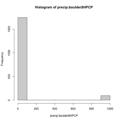
Looking at the histogram, it looks like we have mostly low values (which makes sense) but a few values
up near 1000 -- likely 999.99. We can assign these entries to be NA, the value that
R interprets as no data.
# assing NoData values to NA
precip.boulder$HPCP[precip.boulder$HPCP==999.99] <- NA

# check that NA values were added;
# we can do this by finding the sum of how many NA values there are
sum(is.na(precip.boulder))

## [1] 94
There are 94 NA values in our dataset. This is missing data.
Questions:
- Do we need to worry about the missing data?
- Could they affect our analyses?
This depends on what questions we are asking. Here we are looking at general patterns in the data across 10 years. Since we have just over 3650 days in our entire dataset, missing 94 probably won't affect the general trends we are looking at.
Can you think of a research question where we would need to be concerned about the missing data?
Plot Precipitation Data
Now that we've cleaned up the data, we can view it. To do this we will plot using
ggplot() from the ggplot2 package.
#plot the data
precPlot_hourly <- ggplot(data=precip.boulder,  # the data frame
      aes(DateTime, HPCP)) +   # the variables of interest
      geom_bar(stat="identity") +   # create a bar graph
      xlab("Date") + ylab("Precipitation (Inches)") +  # label the x & y axes
      ggtitle("Hourly Precipitation - Boulder Station\n 2003-2013")  # add a title

precPlot_hourly

## Warning: Removed 94 rows containing missing values (position_stack).
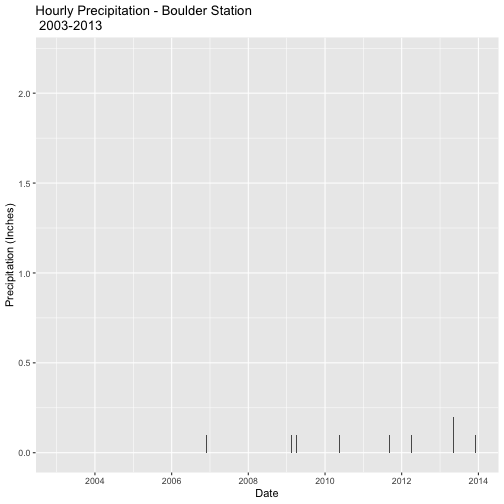
As we can see, plots of hourly date lead to very small numbers and is difficult to represent all information on a figure. Hint: If you can't see any bars on your plot you might need to zoom in on it.
Plots and comparison of daily precipitation would be easier to view.
Plot Daily Precipitation
There are several ways to aggregate the data.
Daily Plots
If you only want to view the data plotted by date you need to create a column with only dates (no time) and then re-plot.
# convert DATE to a Date class
# (this will strip the time, but that is saved in DateTime)
precip.boulder$DATE <- as.Date(precip.boulder$DateTime, # convert to Date class
                                  format="%Y%m%d %H:%M")
                                  #DATE in the format: YearMonthDay Hour:Minute

# double check conversion
str(precip.boulder$DATE)

##  Date[1:1840], format: "2003-01-01" "2003-02-01" "2003-02-03" "2003-02-03" ...

precPlot_daily1 <- ggplot(data=precip.boulder,  # the data frame
      aes(DATE, HPCP)) +   # the variables of interest
      geom_bar(stat="identity") +   # create a bar graph
      xlab("Date") + ylab("Precipitation (Inches)") +  # label the x & y axes
      ggtitle("Daily Precipitation - Boulder Station\n 2003-2013")  # add a title

precPlot_daily1

## Warning: Removed 94 rows containing missing values (position_stack).
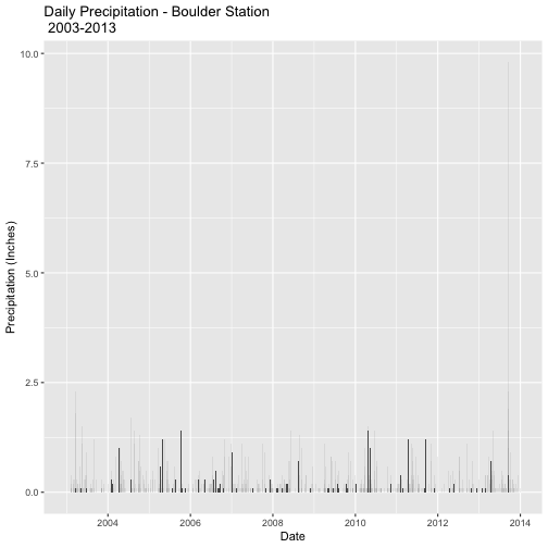
R will automatically combine all data from the same day and plot it as one entry.
Daily Plots & Data
If you want to record the combined hourly data for each day, you need to create a new data frame to store the daily data. We can
use the aggregate() function to combine all the hourly data into daily data.
We will use the date class DATE field we created in the previous code for this.
# aggregate the Precipitation (PRECIP) data by DATE
precip.boulder_daily <-aggregate(precip.boulder$HPCP,   # data to aggregate
	by=list(precip.boulder$DATE),  # variable to aggregate by
	FUN=sum,   # take the sum (total) of the precip
	na.rm=TRUE)  # if the are NA values ignore them
	# if this is FALSE any NA value will prevent a value be totalled

# view the results
head(precip.boulder_daily)

##      Group.1   x
## 1 2003-01-01 0.0
## 2 2003-02-01 0.0
## 3 2003-02-03 0.4
## 4 2003-02-05 0.2
## 5 2003-02-06 0.1
## 6 2003-02-07 0.1
So we now have daily data but the column names don't mean anything. We can
give them meaningful names by using the names() function. Instead of naming the column of
precipitation values with the original HPCP, let's call it PRECIP.
# rename the columns
names(precip.boulder_daily)[names(precip.boulder_daily)=="Group.1"] <- "DATE"
names(precip.boulder_daily)[names(precip.boulder_daily)=="x"] <- "PRECIP"

# double check rename
head(precip.boulder_daily)

##         DATE PRECIP
## 1 2003-01-01    0.0
## 2 2003-02-01    0.0
## 3 2003-02-03    0.4
## 4 2003-02-05    0.2
## 5 2003-02-06    0.1
## 6 2003-02-07    0.1
Now we can plot the daily data.
# plot daily data
precPlot_daily <- ggplot(data=precip.boulder_daily,  # the data frame
      aes(DATE, PRECIP)) +   # the variables of interest
      geom_bar(stat="identity") +   # create a bar graph
      xlab("Date") + ylab("Precipitation (Inches)") +  # label the x & y axes
      ggtitle("Daily Precipitation - Boulder Station\n 2003-2013")  # add a title

precPlot_daily
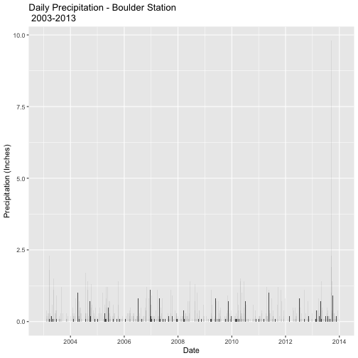
Compare this plot to the plot we created using the first method. Are they the same?
R Tip: This manipulation, or aggregation, of data
can also be done with the package plyr using the summarize() function.
Subset the Data
Instead of looking at the data for the full decade, let's now focus on just the 2 months surrounding the flood on 11-15 September. We'll focus on the window from 15 August to 15 October.
Just like aggregating, we can accomplish this by interacting with the larger plot through the graphical interface or by creating a subset of the data and protting it separately.
Subset Within Plot
To see only a subset of the larger plot, we can simply set limits for the
scale on the x-axis with scale_x_date().
# First, define the limits -- 2 months around the floods
limits <- as.Date(c("2013-08-15", "2013-10-15"))

# Second, plot the data - Flood Time Period
precPlot_flood <- ggplot(data=precip.boulder_daily,
      aes(DATE, PRECIP)) +
      geom_bar(stat="identity") +
      scale_x_date(limits=limits) +
      xlab("Date") + ylab("Precipitation (Inches)") +
      ggtitle("Precipitation - Boulder Station\n August 15 - October 15, 2013")

precPlot_flood

## Warning: Removed 770 rows containing missing values (position_stack).
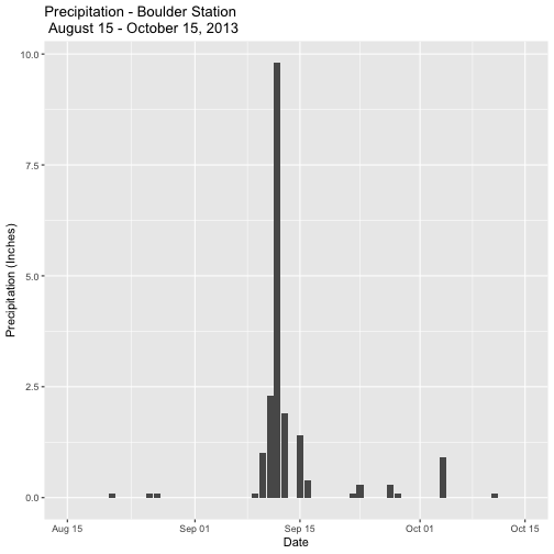
Now we can easily see the dramatic rainfall event in mid-September!
R Tip: If you are using a date-time class, instead
of just a date class, you need to use scale_x_datetime().
Subset The Data
Now let's create a subset of the data and plot it.
# subset 2 months around flood
precip.boulder_AugOct <- subset(precip.boulder_daily,
DATE >= as.Date('2013-08-15') &
DATE <= as.Date('2013-10-15'))
# check the first & last dates
min(precip.boulder_AugOct$DATE)
## [1] "2013-08-21"
max(precip.boulder_AugOct$DATE)
## [1] "2013-10-11"
# create new plot
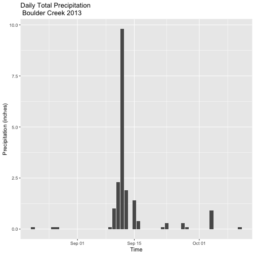
precPlot_flood2 <- ggplot(data=precip.boulder_AugOct, aes(DATE,PRECIP)) +
geom_bar(stat="identity") +
xlab("Time") + ylab("Precipitation (inches)") +
ggtitle("Daily Total Precipitation \n Boulder Creek 2013")
precPlot_flood2
Interactive Plots - Plotly
Let's turn our plot into an interactive Plotly plot.
# setup your plot.ly credentials; if not already set up
#Sys.setenv("plotly_username"="your.user.name.here")
#Sys.setenv("plotly_api_key"="your.key.here")


# view plotly plot in R
ggplotly(precPlot_flood2)


# publish plotly plot to your plot.ly online account when you are happy with it
api_create(precPlot_flood2)
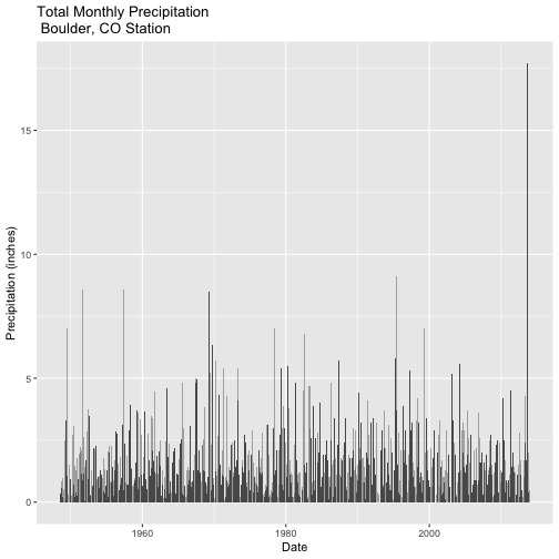
Challenge: Plot Precip for Boulder Station Since 1948
The Boulder precipitation station has been recording data since 1948. Use the steps above to create a plot of the full record of precipitation at this station (1948 - 2013). The full dataset takes considerable time to download, so we recommend you use the dataset provided in the compressed file ("805333-precip_daily_1948-2013.csv").
As an added challenge, aggregate the data by month instead of by day.
Additional Resources
Units & Scale
If you are using a dataset downloaded before 2016, the units were in
hundredths of an inch, this isn't the most useful measure. You might want to
create a new column PRECIP that contains the data from HPCP converted to
inches.
# convert from 100th inch by dividing by 100
precip.boulder$PRECIP<-precip.boulder$HPCP/100

# view & check to make sure conversion occurred
head(precip.boulder)

##       STATION    STATION_NAME ELEVATION LATITUDE LONGITUDE       DATE
## 1 COOP:050843 BOULDER 2 CO US    1650.5 40.03389 -105.2811 2003-01-01
## 2 COOP:050843 BOULDER 2 CO US    1650.5 40.03389 -105.2811 2003-02-01
## 3 COOP:050843 BOULDER 2 CO US    1650.5 40.03389 -105.2811 2003-02-03
## 4 COOP:050843 BOULDER 2 CO US    1650.5 40.03389 -105.2811 2003-02-03
## 5 COOP:050843 BOULDER 2 CO US    1650.5 40.03389 -105.2811 2003-02-03
## 6 COOP:050843 BOULDER 2 CO US    1650.5 40.03389 -105.2811 2003-02-05
##   HPCP Measurement.Flag Quality.Flag            DateTime PRECIP
## 1  0.0                g              2003-01-01 01:00:00  0.000
## 2  0.0                g              2003-02-01 01:00:00  0.000
## 3  0.2                               2003-02-02 19:00:00  0.002
## 4  0.1                               2003-02-02 22:00:00  0.001
## 5  0.1                               2003-02-03 02:00:00  0.001
## 6  0.1                               2003-02-05 02:00:00  0.001
Question
Compare HPCP and PRECIP. Did we do the conversion correctly?