Data Activity: Visualize Stream Discharge Data in R to Better Understand the 2013 Colorado Floods
Authors:
Megan A. Jones, Leah A. Wasser, Mariela Perignon
Last Updated:
Jan 24, 2024
Several factors contributed to the extreme flooding that occurred in Boulder,
Colorado in 2013. In this data activity, we explore and visualize the data for
stream discharge data collected by the United States Geological Survey (USGS).
The tutorial is part of the Data Activities that can be used
with the
Quantifying The Drivers and Impacts of Natural Disturbance Events Teaching Module.
Learning Objectives
After completing this tutorial, you will be able to:
Download stream gauge data from .
Plot precipitation data in R.
Publish & share an interactive plot of the data using Plotly.
Things You'll Need To Complete This Lesson
Please be sure you have the most current version of R and, preferably,
RStudio to write your code.
R Libraries to Install:
ggplot2:install.packages("ggplot2")
plotly:install.packages("plotly")
Data to Download
We include directions on how to directly find and access the data from USGS's
National National Water Information System Database. However, depending on your
learning objectives you may prefer to use the
provided teaching data subset that can be downloaded from the .
Set Working Directory This lesson assumes that you have set your working
directory to the location of the downloaded and unzipped data subsets.
R Script & Challenge Code: NEON data lessons often contain challenges that
reinforce learned skills. If available, the code for challenge solutions is found
in the downloadable R script of the entire lesson, available in the footer of each lesson page.
Research Question
What were the patterns of stream discharge prior to and during the 2013 flooding
events in Colorado?
AGŐćČË°ŮĽŇŔֹٷ˝ÍřŐľ the Data - USGS Stream Discharge Data
The USGS has a distributed network of aquatic sensors located in streams across
the United States. This network monitors a suit of variables that are important
to stream morphology and health. One of the metrics that this sensor network
monitors is Stream Discharge, a metric which quantifies the volume of water
moving down a stream. Discharge is an ideal metric to quantify flow, which
increases significantly during a flood event.
As defined by USGS: Discharge is the volume of water moving down a stream or
river per unit of time, commonly expressed in cubic feet per second or gallons
per day. In general, river discharge is computed by multiplying the area of
water in a channel cross section by the average velocity of the water in that
cross section.
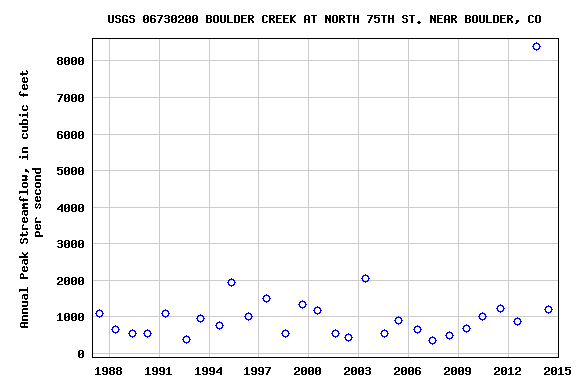
The USGS tracks stream discharge through time at locations across the United
States. Note the pattern observed in the plot above. The peak recorded discharge
value in 2013 was significantly larger than what was observed in other years.
Source:
Obtain USGS Stream Gauge Data
This next section explains how to find and locate data through the USGS's
.
If you want to use the pre-compiled dataset at the FigShare link above, you can skip this
section and start again at the Work With Stream Gauge Data header.
Step 1: Search for the data
To search for stream gauge data in a particular area, we can use the
.
By searching for locations around "Boulder, CO", we can find 3 gauges in the area.
For this lesson, we want data collected by USGS stream gauge 06730200 located on
Boulder Creek at North 75th St. This gauge is one of the few the was able to continuously
collect data throughout the 2013 Boulder floods.
You can directly access the data for this station through the "Access Data" link
on the map icon or searching for this site on the
.
On the
, we can now see summary information about the types of data available for this
station. We want to select Daily Data and then the following parameters:
Available Parameters = 00060 Discharge (Mean)
Output format = Tab-separated
Begin Date = 1 October 1986
End Date = 31 December 2013
Now click "Go".
Step 2: Save data to .txt
The output is a plain text page that you must copy into a spreadsheet of
choice and save as a .csv. Note, you can also download the teaching dataset
(above) or access the data through an API (see Additional Resources, below).
Work with Stream Gauge Data
R Packages
We will use ggplot2 to efficiently plot our data and plotly to create interactive plots.
# load packages

library(ggplot2) # create efficient, professional plots

library(plotly) # create cool interactive plots


## Set your working directory to ensure R can find the file we wish to import and where we want to save our files. Be sure to move the downloaded files into your working directory!

wd <- "~/data/" # This will depend on your local environment

setwd(wd)
Import USGS Stream Discharge Data Into R
Now that we better understand the data that we are working with, let's import it into R. First, open up the discharge/06730200-discharge_daily_1986-2013.txt file in a text editor.
What do you notice about the structure of the file?
The first 24 lines are descriptive text and not actual data. Also notice that this file is separated by tabs, not commas. We will need to specify the
tab delimiter when we import our data.We will use the read.csv() function to import it into an R object.
When we use read.csv(), we need to define several attributes of the file
including:
The data are tab delimited. We will this tell R to use the "\\t"separator, which defines a tab delimited separation.
The first group of 24 lines in the file are not data; we will tell R to skip
those lines when it imports the data using skip=25.
Our data have a header, which is similar to column names in a spreadsheet. We
will tell R to set header=TRUE to ensure the headers are imported as column
names rather than data values.
Finally we will set stringsAsFactors = FALSE to ensure our data come in as individual values.
Let's import our data.
(Note: you can use the discharge/06730200-discharge_daily_1986-2013.csv file
and read it in directly using read.csv() function and then skip to the View
Data Structure section).
#import data

discharge <- read.csv(paste0(wd,"disturb-events-co13/discharge/06730200-discharge_daily_1986-2013.txt"),
                      sep= "\t", skip=24,
                      header=TRUE,
                      stringsAsFactors = FALSE)


#view first few lines

head(discharge)

##   agency_cd  site_no   datetime X17663_00060_00003 X17663_00060_00003_cd
## 1        5s      15s        20d                14n                   10s
## 2      USGS 06730200 1986-10-01                 30                     A
## 3      USGS 06730200 1986-10-02                 30                     A
## 4      USGS 06730200 1986-10-03                 30                     A
## 5      USGS 06730200 1986-10-04                 30                     A
## 6      USGS 06730200 1986-10-05                 30                     A
When we import these data, we can see that the first row of data is a second
header row rather than actual data. We can remove the second row of header
values by selecting all data beginning at row 2 and ending at the
total number or rows in the file and re-assigning it to the variable discharge. The nrow function will count the total
number of rows in the object.
# nrow: how many rows are in the R object

nrow(discharge)

## [1] 9955

# remove the first line from the data frame (which is a second list of headers)

# the code below selects all rows beginning at row 2 and ending at the total

# number of rows.

discharge <- discharge[2:nrow(discharge),]
Metadata
We now have an R object that includes only rows containing data values. Each
column also has a unique column name. However the column names may not be
descriptive enough to be useful - what is X17663_00060_00003?.
Reopen the discharge/06730200-discharge_daily_1986-2013.txt file in a text editor or browser. The text at
the top provides useful metadata about our data. On rows 10-12, we see that the
values in the 5th column of data are "Discharge, cubic feed per second (Mean)". Rows 14-16 tell us more about the 6th column of data,
the quality flags.
Now that we know what the columns are, let's rename column 5, which contains the
discharge value, as disValue and column 6 as qualFlag so it is more "human
readable" as we work with it
in R.
#view structure of data

str(discharge)

## 'data.frame':	9954 obs. of  5 variables:
##  $ agency_cd: chr  "USGS" "USGS" "USGS" "USGS" ...
##  $ site_no  : chr  "06730200" "06730200" "06730200" "06730200" ...
##  $ datetime : chr  "1986-10-01" "1986-10-02" "1986-10-03" "1986-10-04" ...
##  $ disValue : chr  "30" "30" "30" "30" ...
##  $ qualCode : chr  "A" "A" "A" "A" ...
It appears as if the discharge value is a character (chr) class. This is
likely because we had an additional row in our data. Let's convert the discharge
column to a numeric class. In this case, we can reassign that column to be of
class: integer given there are no decimal places.
# view class of the disValue column

class(discharge$disValue)

## [1] "character"

# convert column to integer

discharge$disValue <- as.integer(discharge$disValue)


str(discharge)

## 'data.frame':	9954 obs. of  5 variables:
##  $ agency_cd: chr  "USGS" "USGS" "USGS" "USGS" ...
##  $ site_no  : chr  "06730200" "06730200" "06730200" "06730200" ...
##  $ datetime : chr  "1986-10-01" "1986-10-02" "1986-10-03" "1986-10-04" ...
##  $ disValue : int  30 30 30 30 30 30 30 30 30 31 ...
##  $ qualCode : chr  "A" "A" "A" "A" ...
Converting Time Stamps
We have converted our discharge data to an integer class. However, the time
stamp field, datetime is still a character class.
To work with and efficiently plot time series data, it is best to convert date
and/or time data to a date/time class. As we have both date and time date, we
will use the class POSIXct.
#view class

class(discharge$datetime)

## [1] "character"

#convert to date/time class - POSIX

discharge$datetime <- as.POSIXct(discharge$datetime, tz ="America/Denver")


#recheck data structure

str(discharge)

## 'data.frame':	9954 obs. of  5 variables:
##  $ agency_cd: chr  "USGS" "USGS" "USGS" "USGS" ...
##  $ site_no  : chr  "06730200" "06730200" "06730200" "06730200" ...
##  $ datetime : POSIXct, format: "1986-10-01" "1986-10-02" "1986-10-03" ...
##  $ disValue : int  30 30 30 30 30 30 30 30 30 31 ...
##  $ qualCode : chr  "A" "A" "A" "A" ...
No Data Values
Next, let's query our data to check whether there are no data values in
it. The metadata associated with the data doesn't specify what the values would
be, NA or -9999 are common values
# check total number of NA values
sum(is.na(discharge$datetime))
## [1] 0
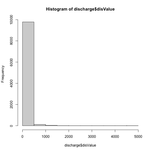
# check for "strange" values that could be an NA indicator
hist(discharge$disValue)
Excellent! The data contains no NoData values.
Plot The Data
Finally, we are ready to plot our data. We will use ggplot from the ggplot2
package to create our plot.
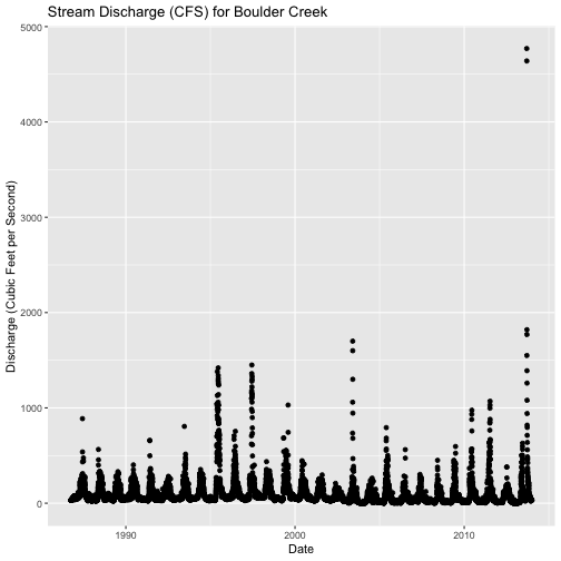
ggplot(discharge, aes(datetime, disValue)) +
  geom_point() +
  ggtitle("Stream Discharge (CFS) for Boulder Creek") +
  xlab("Date") + ylab("Discharge (Cubic Feet per Second)")
Questions:
What patterns do you see in the data?
Why might there be an increase in discharge during a particular time of year?
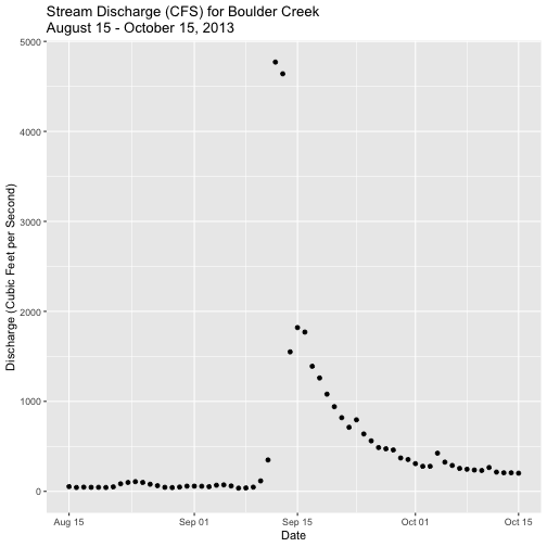
Plot Data Time Subsets With ggplot
We can plot a subset of our data within ggplot() by specifying the start and
end times (in a limits object) for the x-axis with scale_x_datetime. Let's
plot data for the months directly around the Boulder flood: August 15 2013 -
October 15 2013.
# Define Start and end times for the subset as R objects that are the time class

start.end <- as.POSIXct(c("2013-08-15 00:00:00","2013-10-15 00:00:00"),tz= "America/Denver")


# plot the data - Aug 15-October 15

ggplot(discharge,
      aes(datetime,disValue)) +
      geom_point() +
      scale_x_datetime(limits=start.end) +
      xlab("Date") + ylab("Discharge (Cubic Feet per Second)") +
      ggtitle("Stream Discharge (CFS) for Boulder Creek\nAugust 15 - October 15, 2013")

## Warning: Removed 9892 rows containing missing values (`geom_point()`).
We get a warning message because we are "ignoring" lots of the data in the
dataset.
Plotly - Interactive (and Online) Plots
We have now successfully created a plot. We can turn that plot into an interactive
plot using Plotly.
allows you to create interactive plots that can also be shared online. If
you are new to Plotly, view the companion mini-lesson
Interactive Data Vizualization with R and Plotly
to learn how to set up an account and access your username and API key.
Time subsets in plotly
To plot a subset of the total data we have to manually subset the data as the Plotly
package doesn't (yet?) recognize the limits method of subsetting.
Here we create a new R object with entries corresponding to just the dates we want and then plot that data.
# subset out some of the data - Aug 15 - October 15

discharge.aug.oct2013 <- subset(discharge,

                        datetime >= as.POSIXct('2013-08-15 00:00',

                                              tz = "America/Denver") &

                        datetime <= as.POSIXct('2013-10-15 23:59',

                                              tz = "America/Denver"))


# plot the data

disPlot.plotly <- ggplot(data=discharge.aug.oct2013,

        aes(datetime,disValue)) +

        geom_point(size=3)     # makes the points larger than default


disPlot.plotly


# add title and labels

disPlot.plotly <- disPlot.plotly +

	theme(axis.title.x = element_blank()) +

	xlab("Time") + ylab("Stream Discharge (CFS)") +

	ggtitle("Stream Discharge - Boulder Creek 2013")


disPlot.plotly
You can now display your interactive plot in R using the following command:
# view plotly plot in R

ggplotly(disPlot.plotly)
If you are satisfied with your plot you can now publish it to your Plotly account, if desired.
# set username

Sys.setenv("plotly_username"="yourUserNameHere")

# set user key

Sys.setenv("plotly_api_key"="yourUserKeyHere")


# publish plotly plot to your plotly online account if you want.

api_create(disPlot.plotly)
Additional Resources
Additional information on USGS streamflow measurements and data:
API Data Access
USGS data can be downloaded via an API using a command line interface. This is
particularly useful if you want to request data from multiple sites or build the
data request into a script.
.