Tutorial
Time Series 00: Intro to Time Series Data in R - Managing Date/Time Formats
Last Updated: May 13, 2021
This tutorial will demonstrate how to import a time series dataset stored in .csv
format into R. It will explore data classes for columns in a data.frame and
will walk through how to
convert a date, stored as a character string, into a date class that R can
recognize and plot efficiently.
Learning Objectives
After completing this tutorial, you will be able to:
- Open a
.csvfile in R usingread.csv()and understand why we are using that file type. - Work with data stored in different columns within a
data.framein R. - Examine R object structures and data
classes. - Convert dates, stored as a character class, into an R date class.
- Create a quick plot of a time-series dataset using
qplot.
Things You’ll Need To Complete This Tutorial
You will need the most current version of R and, preferably, RStudio loaded on your computer to complete this tutorial.
Install R Packages
-
ggplot2:
install.packages("ggplot2")
More on Packages in R � Adapted from Software Carpentry.
Download Data
The data used in this lesson were collected at the National Ecological Observatory Network's Harvard Forest field site. These data are proxy data for what will be available for 30 years on the for the Harvard Forest and other field sites located across the United States.
Set Working Directory: This lesson assumes that you have set your working directory to the location of the downloaded and unzipped data subsets.
An overview of setting the working directory in R can be found here.
R Script & Challenge Code: NEON data lessons often contain challenges that reinforce learned skills. If available, the code for challenge solutions is found in the downloadable R script of the entire lesson, available in the footer of each lesson page.
Data Related to Phenology
In this tutorial, we will explore atmospheric data (including temperature, precipitation and other metrics) collected by sensors mounted on a flux tower at the NEON Harvard Forest field site. We are interested in exploring changes in temperature, precipitation, Photosynthetically Active Radiation (PAR) and day length throughout the year -- metrics that impact changes in the timing of plant .
AGŐćČË°ŮĽŇŔֹٷ˝ÍřŐľ .csv Format
The data that we will use is in .csv (comma-separated values) file format. The
.csv format is a plain text format, where each value in the dataset is
separate by a comma and each "row" in the dataset is separated by a line break.
Plain text formats are ideal for working both across platforms (Mac, PC, LINUX,
etc) and also can be read by many different tools. The plain text
format is also less likely to become obsolete over time.
Import the Data
To begin, let's import the data into R. We can use base R functionality
to import a .csv file. We will use the ggplot2 package to plot our data.
# Load packages required for entire script.
# library(PackageName)  # purpose of package
library(ggplot2)   # efficient, pretty plotting - required for qplot function

# set working directory to ensure R can find the file we wish to import
# provide the location for where you've unzipped the lesson data
wd <- "~/Git/data/"
Once our working directory is set, we can import the file using read.csv().
# Load csv file of daily meteorological data from Harvard Forest
harMet.daily <- read.csv(
      file=paste0(wd,"NEON-DS-Met-Time-Series/HARV/FisherTower-Met/hf001-06-daily-m.csv"),
      stringsAsFactors = FALSE
      )
stringsAsFactors=FALSE
When reading in files we most often use stringsAsFactors = FALSE. This
setting ensures that non-numeric data (strings) are not converted to
factors.
What Is A Factor?
A factor is similar to a category. However factors can be numerically interpreted (they can have an order) and may have a level associated with them.
Examples of factors:
- Month Names (an ordinal variable): Month names are non-numerical but we know that April (month 4) comes after March (month 3) and each could be represented by a number (4 & 3).
- 1 and 2s to represent male and female sex (a nominal variable): Numerical interpretation of non-numerical data but no order to the levels.
After loading the data it is easy to convert any field that should be a factor by
using as.factor(). Therefore it is often best to read in a file with
stringsAsFactors = FALSE.
Data.Frames in R
The read.csv() imports our .csv into a data.frame object in R. data.frames
are ideal for working with tabular data - they are similar to a spreadsheet.
# what type of R object is our imported data?
class(harMet.daily)

## [1] "data.frame"
Data Structure
Once the data are imported, we can explore their structure. There are several ways to examine the structure of a data frame:
-
head(): shows us the first 6 rows of the data (tail()shows the last 6 rows). -
str(): displays the structure of the data as R interprets it.
Let's use both to explore our data.
# view first 6 rows of the dataframe
head(harMet.daily)

##         date jd  airt f.airt airtmax f.airtmax airtmin f.airtmin rh
## 1 2001-02-11 42 -10.7           -6.9             -15.1           40
## 2 2001-02-12 43  -9.8           -2.4             -17.4           45
## 3 2001-02-13 44  -2.0            5.7              -7.3           70
## 4 2001-02-14 45  -0.5            1.9              -5.7           78
## 5 2001-02-15 46  -0.4            2.4              -5.7           69
## 6 2001-02-16 47  -3.0            1.3              -9.0           82
##   f.rh rhmax f.rhmax rhmin f.rhmin  dewp f.dewp dewpmax f.dewpmax
## 1         58            22         -22.2          -16.8
## 2         85            14         -20.7           -9.2
## 3        100            34          -7.6           -4.6
## 4        100            59          -4.1            1.9
## 5        100            37          -6.0            2.0
## 6        100            46          -5.9           -0.4
##   dewpmin f.dewpmin prec f.prec slrt f.slrt part f.part netr f.netr
## 1   -25.7            0.0        14.9          NA      M   NA      M
## 2   -27.9            0.0        14.8          NA      M   NA      M
## 3   -10.2            0.0        14.8          NA      M   NA      M
## 4   -10.2            6.9         2.6          NA      M   NA      M
## 5   -12.1            0.0        10.5          NA      M   NA      M
## 6   -10.6            2.3         6.4          NA      M   NA      M
##    bar f.bar wspd f.wspd wres f.wres wdir f.wdir wdev f.wdev gspd
## 1 1025        3.3         2.9         287          27        15.4
## 2 1033        1.7         0.9         245          55         7.2
## 3 1024        1.7         0.9         278          53         9.6
## 4 1016        2.5         1.9         197          38        11.2
## 5 1010        1.6         1.2         300          40        12.7
## 6 1016        1.1         0.5         182          56         5.8
##   f.gspd s10t f.s10t s10tmax f.s10tmax s10tmin f.s10tmin
## 1          NA      M      NA         M      NA         M
## 2          NA      M      NA         M      NA         M
## 3          NA      M      NA         M      NA         M
## 4          NA      M      NA         M      NA         M
## 5          NA      M      NA         M      NA         M
## 6          NA      M      NA         M      NA         M

# View the structure (str) of the data
str(harMet.daily)

## 'data.frame':	5345 obs. of  46 variables:
##  $ date     : chr  "2001-02-11" "2001-02-12" "2001-02-13" "2001-02-14" ...
##  $ jd       : int  42 43 44 45 46 47 48 49 50 51 ...
##  $ airt     : num  -10.7 -9.8 -2 -0.5 -0.4 -3 -4.5 -9.9 -4.5 3.2 ...
##  $ f.airt   : chr  "" "" "" "" ...
##  $ airtmax  : num  -6.9 -2.4 5.7 1.9 2.4 1.3 -0.7 -3.3 0.7 8.9 ...
##  $ f.airtmax: chr  "" "" "" "" ...
##  $ airtmin  : num  -15.1 -17.4 -7.3 -5.7 -5.7 -9 -12.7 -17.1 -11.7 -1.3 ...
##  $ f.airtmin: chr  "" "" "" "" ...
##  $ rh       : int  40 45 70 78 69 82 66 51 57 62 ...
##  $ f.rh     : chr  "" "" "" "" ...
##  $ rhmax    : int  58 85 100 100 100 100 100 71 81 78 ...
##  $ f.rhmax  : chr  "" "" "" "" ...
##  $ rhmin    : int  22 14 34 59 37 46 30 34 37 42 ...
##  $ f.rhmin  : chr  "" "" "" "" ...
##  $ dewp     : num  -22.2 -20.7 -7.6 -4.1 -6 -5.9 -10.8 -18.5 -12 -3.5 ...
##  $ f.dewp   : chr  "" "" "" "" ...
##  $ dewpmax  : num  -16.8 -9.2 -4.6 1.9 2 -0.4 -0.7 -14.4 -4 0.6 ...
##  $ f.dewpmax: chr  "" "" "" "" ...
##  $ dewpmin  : num  -25.7 -27.9 -10.2 -10.2 -12.1 -10.6 -25.4 -25 -16.5 -5.7 ...
##  $ f.dewpmin: chr  "" "" "" "" ...
##  $ prec     : num  0 0 0 6.9 0 2.3 0 0 0 0 ...
##  $ f.prec   : chr  "" "" "" "" ...
##  $ slrt     : num  14.9 14.8 14.8 2.6 10.5 6.4 10.3 15.5 15 7.7 ...
##  $ f.slrt   : chr  "" "" "" "" ...
##  $ part     : num  NA NA NA NA NA NA NA NA NA NA ...
##  $ f.part   : chr  "M" "M" "M" "M" ...
##  $ netr     : num  NA NA NA NA NA NA NA NA NA NA ...
##  $ f.netr   : chr  "M" "M" "M" "M" ...
##  $ bar      : int  1025 1033 1024 1016 1010 1016 1008 1022 1022 1017 ...
##  $ f.bar    : chr  "" "" "" "" ...
##  $ wspd     : num  3.3 1.7 1.7 2.5 1.6 1.1 3.3 2 2.5 2 ...
##  $ f.wspd   : chr  "" "" "" "" ...
##  $ wres     : num  2.9 0.9 0.9 1.9 1.2 0.5 3 1.9 2.1 1.8 ...
##  $ f.wres   : chr  "" "" "" "" ...
##  $ wdir     : int  287 245 278 197 300 182 281 272 217 218 ...
##  $ f.wdir   : chr  "" "" "" "" ...
##  $ wdev     : int  27 55 53 38 40 56 24 24 31 27 ...
##  $ f.wdev   : chr  "" "" "" "" ...
##  $ gspd     : num  15.4 7.2 9.6 11.2 12.7 5.8 16.9 10.3 11.1 10.9 ...
##  $ f.gspd   : chr  "" "" "" "" ...
##  $ s10t     : num  NA NA NA NA NA NA NA NA NA NA ...
##  $ f.s10t   : chr  "M" "M" "M" "M" ...
##  $ s10tmax  : num  NA NA NA NA NA NA NA NA NA NA ...
##  $ f.s10tmax: chr  "M" "M" "M" "M" ...
##  $ s10tmin  : num  NA NA NA NA NA NA NA NA NA NA ...
##  $ f.s10tmin: chr  "M" "M" "M" "M" ...
Classes in R
The structure results above let us know that the attributes in our data.frame
are stored as several different data types or classes as follows:
- chr - Character: It holds strings that are composed of letters and words. Character class data can not be interpreted numerically - that is to say we can not perform math on these values even if they contain only numbers.
- int - Integer: It holds numbers that are whole integers without decimals. Mathematical operations can be performed on integers.
- num - Numeric: It accepts data that are a wide variety of numeric formats including decimals (floating point values) and integers. Numeric also accept larger numbers than int will.
Storing variables using different classes is a strategic decision by R (and
other programming languages) that optimizes processing and storage. It allows:
- data to be processed more quickly & efficiently.
- the program (R) to minimize the storage size.
Differences Between Classes
Certain functions can be performed on certain data classes and not on others.
For example:
a <- "mouse"
b <- "sparrow"
class(a)

## [1] "character"

class(b)

## [1] "character"

# subtract a-b
a-b

## Error in a - b: non-numeric argument to binary operator
You can not subtract two character values given they are not numbers.
c <- 2
d <- 1
class(c)

## [1] "numeric"

class(d)

## [1] "numeric"

# subtract a-b
c-d

## [1] 1
Additionally, performing summary statistics and other calculations of different types of classes can yield different results.
# create a new object
speciesObserved <- c("speciesb","speciesc","speciesa")
speciesObserved

## [1] "speciesb" "speciesc" "speciesa"

# determine the class
class(speciesObserved)

## [1] "character"

# calculate the minimum
min(speciesObserved)

## [1] "speciesa"

# create numeric object
prec <- c(1,2,5,3,6)
# view class
class(prec)

## [1] "numeric"

# calculate min value
min(prec)

## [1] 1
We can calculate the minimum value for SpeciesObserved, a character
data class, however it does not return a quantitative minimum. It simply
looks for the first element, using alphabetical (rather than numeric) order.
Yet, we can calculate the quantitative minimum value for prec a numeric
data class.
Plot Data Using qplot()
Now that we've got classes down, let's plot one of the metrics in our data,
air temperature -- airt. Given this is a time series dataset, we want to plot
air temperature as it changes over time. We have a date-time column, date, so
let's use that as our x-axis variable and airt as our y-axis variable.
We will use the qplot() (for quick plot) function in the ggplot2 package.
The syntax for qplot() requires the x- and y-axis variables and then the R
object that the variables are stored in.
# quickly plot air temperature
qplot(x=date, y=airt,
      data=harMet.daily,
      main="Daily Air Temperature\nNEON Harvard Forest Field Site")
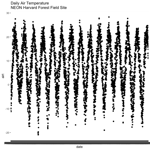
We have successfully plotted some data. However, what is happening on the x-axis?
R is trying to plot EVERY date value in our data, on the x-axis. This makes it hard to read. Why? Let's have a look at the class of the x-axis variable - date.
# View data class for each column that we wish to plot
class(harMet.daily$date)

## [1] "character"

class(harMet.daily$airt)

## [1] "numeric"
In this case, the date column is stored in our data.frame as a character
class. Because it is a character, R does not know how to plot the dates as a
continuous variable. Instead it tries to plot every date value as a text string.
The airt data class is numeric so that metric plots just fine.
Date as a Date-Time Class
We need to convert our date column, which is currently stored as a character
to a date-time class that can be displayed as a continuous variable. Lucky
for us, R has a date class. We can convert the date field to a date class
using as.Date().
# convert column to date class
harMet.daily$date <- as.Date(harMet.daily$date)

# view R class of data
class(harMet.daily$date)

## [1] "Date"

# view results
head(harMet.daily$date)

## [1] "2001-02-11" "2001-02-12" "2001-02-13" "2001-02-14" "2001-02-15"
## [6] "2001-02-16"
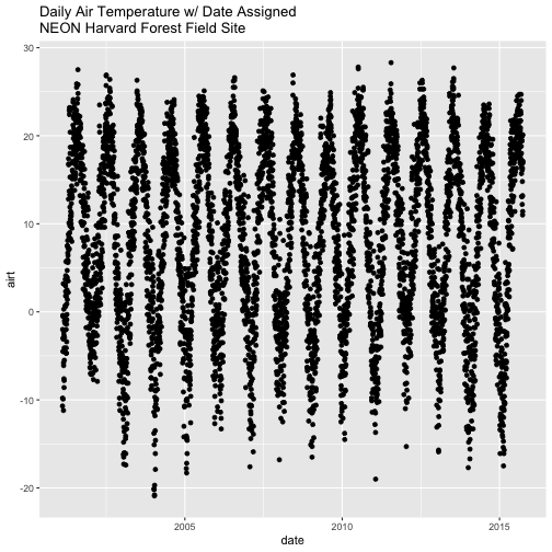
Now that we have adjusted the date, let's plot again. Notice that it plots
much more quickly now that R recognizes date as a date class. R can
aggregate ticks on the x-axis by year instead of trying to plot every day!
# quickly plot the data and include a title using main=""
# In title string we can use '\n' to force the string to break onto a new line
qplot(x=date,y=airt,
      data=harMet.daily,
      main="Daily Air Temperature w/ Date Assigned\nNEON Harvard Forest Field Site")
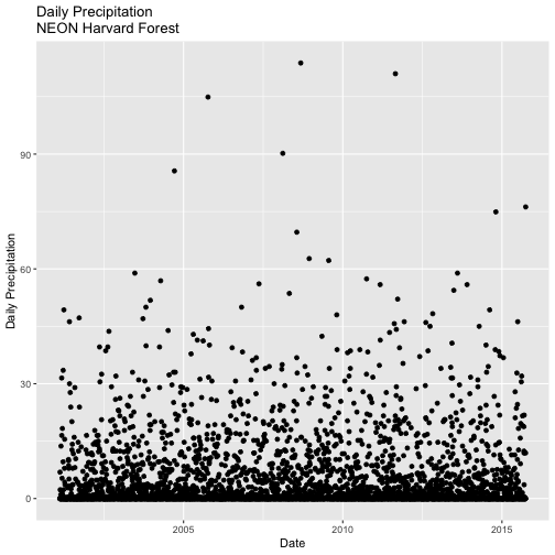
- Create a quick plot of the precipitation. Use the full time frame of data available
in the
harMet.dailyobject. - Do precipitation and air temperature have similar annual patterns?
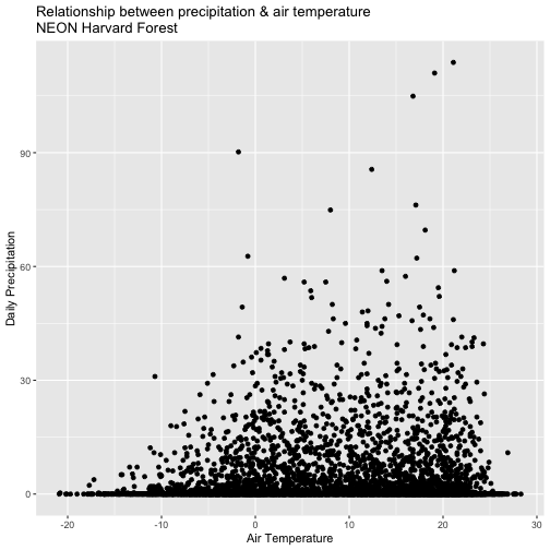
- Create a quick plot examining the relationship between air temperature and precipitation.
Hint: you can modify the X and Y axis labels using xlab="label text" and
ylab="label text".