Tutorial
Vector 04: Convert from .csv to a Shapefile in R
Last Updated: Apr 8, 2021
This tutorial will review how to import spatial points stored in .csv (Comma
Separated Value) format into
R as a spatial object - a SpatialPointsDataFrame. We will also
reproject data imported in a shapefile format, export a shapefile from an
R spatial object, and plot raster and vector data as
layers in the same plot.
Learning Objectives
After completing this tutorial, you will be able to:
- Import .csv files containing x,y coordinate locations into R.
- Convert a .csv to a spatial object.
- Project coordinate locations provided in a Geographic Coordinate System (Latitude, Longitude) to a projected coordinate system (UTM).
- Plot raster and vector data in the same plot to create a map.
Things You’ll Need To Complete This Tutorial
You will need the most current version of R and, preferably, RStudio loaded
on your computer to complete this tutorial.
Install R Packages
-
raster:
install.packages("raster") -
rgdal:
install.packages("rgdal") -
sp:
install.packages("sp") -
More on Packages in R � Adapted from Software Carpentry.
Data to Download
These vector data provide information on the site characterization and infrastructure at the National Ecological Observatory Network's Harvard Forest field site. The Harvard Forest shapefiles are from the archives. US Country and State Boundary layers are from the .
The LiDAR and imagery data used to create this raster teaching data subset were collected over the National Ecological Observatory Network's Harvard Forest and San Joaquin Experimental Range field sites and processed at NEON headquarters. The entire dataset can be accessed by request from the .
Set Working Directory: This lesson assumes that you have set your working directory to the location of the downloaded and unzipped data subsets.
An overview of setting the working directory in R can be found here.
R Script & Challenge Code: NEON data lessons often contain challenges that reinforce learned skills. If available, the code for challenge solutions is found in the downloadable R script of the entire lesson, available in the footer of each lesson page.
Spatial Data in Text Format
The HARV_PlotLocations.csv file contains x, y (point) locations for study
plots where NEON collects data on
vegetation and other ecological metrics.
We would like to:
- Create a map of these plot locations.
- Export the data in a
shapefileformat to share with our colleagues. This shapefile can be imported into any GIS software. - Create a map showing vegetation height with plot locations layered on top.
Spatial data are sometimes stored in a text file format (.txt or .csv). If
the text file has an associated x and y location column, then we can
convert it into an R spatial object, which, in the case of point data,
will be a SpatialPointsDataFrame. The SpatialPointsDataFrame
allows us to store both the x,y values that represent the coordinate location
of each point and the associated attribute data, or columns describing each
feature in the spatial object.
We will use the rgdal and raster libraries in this tutorial.
# load packages
library(rgdal)  # for vector work; sp package should always load with rgdal
library (raster)   # for metadata/attributes- vectors or rasters

# set working directory to data folder
# setwd("pathToDirHere")
Import .csv
To begin let's import the .csv file that contains plot coordinate x, y
locations at the NEON Harvard Forest Field Site (HARV_PlotLocations.csv) into
R. Note that we set stringsAsFactors=FALSE so our data imports as a
character rather than a factor class.
# Read the .csv file
plot.locations_HARV <-
  read.csv("NEON-DS-Site-Layout-Files/HARV/HARV_PlotLocations.csv",
           stringsAsFactors = FALSE)

# look at the data structure
str(plot.locations_HARV)

## 'data.frame':	21 obs. of  16 variables:
##  $ easting   : num  731405 731934 731754 731724 732125 ...
##  $ northing  : num  4713456 4713415 4713115 4713595 4713846 ...
##  $ geodeticDa: chr  "WGS84" "WGS84" "WGS84" "WGS84" ...
##  $ utmZone   : chr  "18N" "18N" "18N" "18N" ...
##  $ plotID    : chr  "HARV_015" "HARV_033" "HARV_034" "HARV_035" ...
##  $ stateProvi: chr  "MA" "MA" "MA" "MA" ...
##  $ county    : chr  "Worcester" "Worcester" "Worcester" "Worcester" ...
##  $ domainName: chr  "Northeast" "Northeast" "Northeast" "Northeast" ...
##  $ domainID  : chr  "D01" "D01" "D01" "D01" ...
##  $ siteID    : chr  "HARV" "HARV" "HARV" "HARV" ...
##  $ plotType  : chr  "distributed" "tower" "tower" "tower" ...
##  $ subtype   : chr  "basePlot" "basePlot" "basePlot" "basePlot" ...
##  $ plotSize  : int  1600 1600 1600 1600 1600 1600 1600 1600 1600 1600 ...
##  $ elevation : num  332 342 348 334 353 ...
##  $ soilTypeOr: chr  "Inceptisols" "Inceptisols" "Inceptisols" "Histosols" ...
##  $ plotdim_m : int  40 40 40 40 40 40 40 40 40 40 ...
Also note that plot.locations_HARV is a data.frame that contains 21
locations (rows) and 15 variables (attributes).
Next, let's explore data.frame to determine whether it contains
columns with coordinate values. If we are lucky, our .csv will contain columns
labeled:
- "X" and "Y" OR
- Latitude and Longitude OR
- easting and northing (UTM coordinates)
Let's check out the column names of our file to look for these.
# view column names
names(plot.locations_HARV)

##  [1] "easting"    "northing"   "geodeticDa" "utmZone"    "plotID"
##  [6] "stateProvi" "county"     "domainName" "domainID"   "siteID"
## [11] "plotType"   "subtype"    "plotSize"   "elevation"  "soilTypeOr"
## [16] "plotdim_m"
Identify X,Y Location Columns
View the column names, we can see that our data.frame that contains several
fields that might contain spatial information. The plot.locations_HARV$easting
and plot.locations_HARV$northing columns contain these coordinate values.
# view first 6 rows of the X and Y columns
head(plot.locations_HARV$easting)

## [1] 731405.3 731934.3 731754.3 731724.3 732125.3 731634.3

head(plot.locations_HARV$northing)

## [1] 4713456 4713415 4713115 4713595 4713846 4713295

# note that  you can also call the same two columns using their COLUMN NUMBER
# view first 6 rows of the X and Y columns
head(plot.locations_HARV[,1])

## [1] 731405.3 731934.3 731754.3 731724.3 732125.3 731634.3

head(plot.locations_HARV[,2])

## [1] 4713456 4713415 4713115 4713595 4713846 4713295
So, we have coordinate values in our data.frame but in order to convert our
data.frame to a SpatialPointsDataFrame, we also need to know the CRS
associated with these coordinate values.
There are several ways to figure out the CRS of spatial data in text format.
- We can check the file metadata in hopes that the CRS was recorded in the data. For more information on metadata, check out the Why Metadata Are Important: How to Work with Metadata in Text & EML Format tutorial.
- We can explore the file itself to see if CRS information is embedded in the file header or somewhere in the data columns.
Following the easting and northing columns, there is a geodeticDa and a
utmZone column. These appear to contain CRS information
(datum and projection), so let's view those next.
# view first 6 rows of the X and Y columns
head(plot.locations_HARV$geodeticDa)

## [1] "WGS84" "WGS84" "WGS84" "WGS84" "WGS84" "WGS84"

head(plot.locations_HARV$utmZone)

## [1] "18N" "18N" "18N" "18N" "18N" "18N"
It is not typical to store CRS information in a column, but this particular
file contains CRS information this way. The geodeticDa and utmZone columns
contain the information that helps us determine the CRS:
-
geodeticDa: WGS84 -- this is geodetic datum WGS84 -
utmZone: 18
In
When Vector Data Don't Line Up - Handling Spatial Projection & CRS in R tutorial
we learned about the components of a proj4 string. We have everything we need
to now assign a CRS to our data.frame.
To create the proj4 associated with UTM Zone 18 WGS84 we could look up the
projection on the
which contains a list of CRS formats for each projection:
- This link shows .
However, if we have other data in the UTM Zone 18N projection, it's much
easier to simply assign the crs() in proj4 format from that object to our
new spatial object. Let's import the roads layer from Harvard forest and check
out its CRS.
Note: if you do not have a CRS to borrow from another raster, see Option 2 in the next section for how to convert to a spatial object and assign a CRS.
# Import the line shapefile
lines_HARV <- readOGR( "NEON-DS-Site-Layout-Files/HARV/", "HARV_roads")

## OGR data source with driver: ESRI Shapefile
## Source: "/Users/olearyd/Git/data/NEON-DS-Site-Layout-Files/HARV", layer: "HARV_roads"
## with 13 features
## It has 15 fields

# view CRS
crs(lines_HARV)

## CRS arguments:
##  +proj=utm +zone=18 +datum=WGS84 +units=m +no_defs

# view extent
extent(lines_HARV)

## class      : Extent
## xmin       : 730741.2
## xmax       : 733295.5
## ymin       : 4711942
## ymax       : 4714260
Exploring the data above, we can see that the lines shapefile is in
UTM zone 18N. We can thus use the CRS from that spatial object to convert our
non-spatial data.frame into a spatialPointsDataFrame.
Next, let's create a crs object that we can use to define the CRS of our
SpatialPointsDataFrame when we create it.
# create crs object
utm18nCRS <- crs(lines_HARV)
utm18nCRS

## CRS arguments:
##  +proj=utm +zone=18 +datum=WGS84 +units=m +no_defs

class(utm18nCRS)

## [1] "CRS"
## attr(,"package")
## [1] "sp"
.csv to R SpatialPointsDataFrame
Let's convert our data.frame into a SpatialPointsDataFrame. To do
this, we need to specify:
- The columns containing X (
easting) and Y (northing) coordinate values - The CRS that the column coordinate represent (units are included in the CRS).
- Optional: the other columns stored in the data frame that you wish to append as attributes to your spatial object.
We can add the CRS in two ways; borrow the CRS from another raster that
already has it assigned (Option 1) or to add it directly using the proj4string
(Option 2).
Option 1: Borrow CRS
We will use the SpatialPointsDataFrame() function to perform the conversion
and add the CRS from our utm18nCRS object.
# note that the easting and northing columns are in columns 1 and 2
plot.locationsSp_HARV <- SpatialPointsDataFrame(plot.locations_HARV[,1:2],
                    plot.locations_HARV,    #the R object to convert
                    proj4string = utm18nCRS)   # assign a CRS

# look at CRS
crs(plot.locationsSp_HARV)

## CRS arguments:
##  +proj=utm +zone=18 +datum=WGS84 +units=m +no_defs
Option 2: Assigning CRS
If we didn't have a raster from which to borrow the CRS, we can directly assign it using either of two equivalent, but slightly different syntaxes.
# first, convert the data.frame to spdf
r <- SpatialPointsDataFrame(plot.locations_HARV[,1:2],
                    plot.locations_HARV)

# second, assign the CRS in one of two ways
r <- crs("+proj=utm +zone=18 +datum=WGS84 +units=m +no_defs
				 +ellps=WGS84 +towgs84=0,0,0" )
# or

crs(r) <- "+proj=utm +zone=18 +datum=WGS84 +units=m +no_defs
				 +ellps=WGS84 +towgs84=0,0,0"
Plot Spatial Object
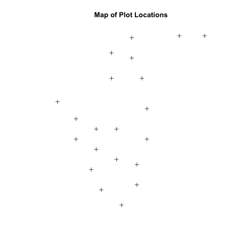
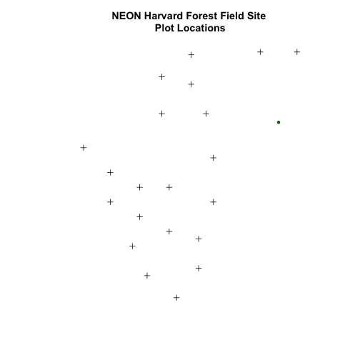
We now have a spatial R object, we can plot our newly created spatial object.
# plot spatial object
plot(plot.locationsSp_HARV,
     main="Map of Plot Locations")
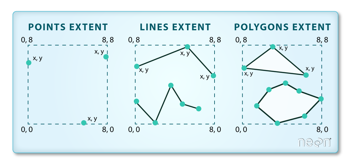
Define Plot Extent
In
Open and Plot Shapefiles in R
we learned about spatial object extent. When we plot several spatial layers in
R, the first layer that is plotted becomes the extent of the plot. If we add
additional layers that are outside of that extent, then the data will not be
visible in our plot. It is thus useful to know how to set the spatial extent of
a plot using xlim and ylim.
Let's first create a SpatialPolygon object from the
NEON-DS-Site-Layout-Files/HarClip_UTMZ18 shapefile. (If you have completed
Vector 00-02 tutorials in this
Introduction to Working with Vector Data in R
series, you can skip this code as you have already created this object.)
# create boundary object
aoiBoundary_HARV <- readOGR("NEON-DS-Site-Layout-Files/HARV/",
                            "HarClip_UTMZ18")

## OGR data source with driver: ESRI Shapefile
## Source: "/Users/olearyd/Git/data/NEON-DS-Site-Layout-Files/HARV", layer: "HarClip_UTMZ18"
## with 1 features
## It has 1 fields
## Integer64 fields read as strings:  id
To begin, let's plot our aoiBoundary object with our vegetation plots.
# plot Boundary
plot(aoiBoundary_HARV,
     main="AOI Boundary\nNEON Harvard Forest Field Site")

# add plot locations
plot(plot.locationsSp_HARV,
     pch=8, add=TRUE)
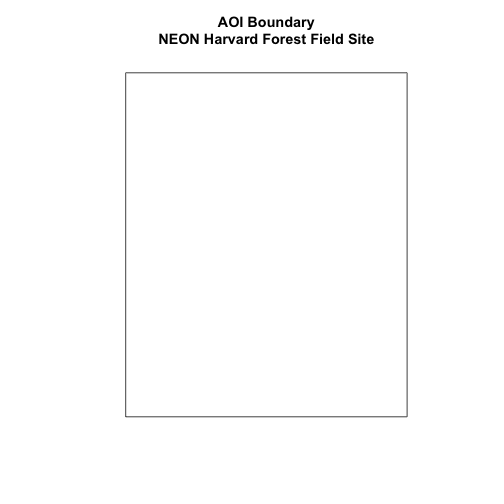
# no plots added, why? CRS?
# view CRS of each
crs(aoiBoundary_HARV)

## CRS arguments:
##  +proj=utm +zone=18 +datum=WGS84 +units=m +no_defs

crs(plot.locationsSp_HARV)

## CRS arguments:
##  +proj=utm +zone=18 +datum=WGS84 +units=m +no_defs
When we attempt to plot the two layers together, we can see that the plot locations are not rendered. Our data are in the same projection, so what is going on?
# view extent of each
extent(aoiBoundary_HARV)
## class : Extent
## xmin : 732128
## xmax : 732251.1
## ymin : 4713209
## ymax : 4713359
extent(plot.locationsSp_HARV)
## class : Extent
## xmin : 731405.3
## xmax : 732275.3
## ymin : 4712845
## ymax : 4713846
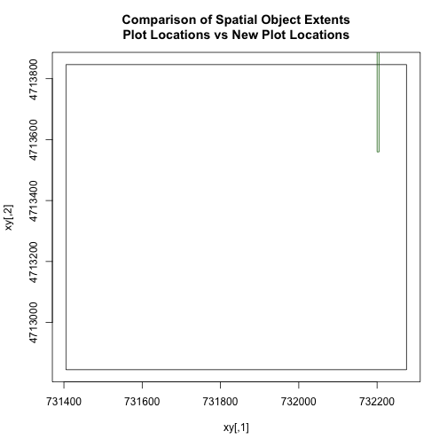
# add extra space to right of plot area;
# par(mar=c(5.1, 4.1, 4.1, 8.1), xpd=TRUE)
plot(extent(plot.locationsSp_HARV),
col="purple",
xlab="easting",
ylab="northing", lwd=8,
main="Extent Boundary of Plot Locations \nCompared to the AOI Spatial Object",
ylim=c(4712400,4714000)) # extent the y axis to make room for the legend
plot(extent(aoiBoundary_HARV),
add=TRUE,
lwd=6,
col="springgreen")
legend("bottomright",
#inset=c(-0.5,0),
legend=c("Layer One Extent", "Layer Two Extent"),
bty="n",
col=c("purple","springgreen"),
cex=.8,
lty=c(1,1),
lwd=6)
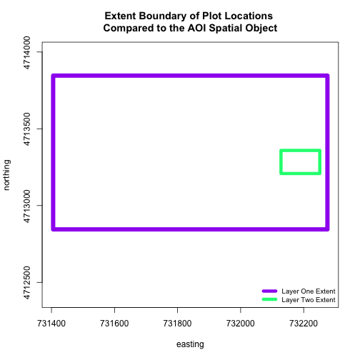
The extents of our two objects are different. plot.locationsSp_HARV is
much larger than aoiBoundary_HARV. When we plot aoiBoundary_HARV first, R
uses the extent of that object to as the plot extent. Thus the points in the
plot.locationsSp_HARV object are not rendered. To fix this, we can manually
assign the plot extent using xlims and ylims. We can grab the extent
values from the spatial object that has a larger extent. Let's try it.
plotLoc.extent <- extent(plot.locationsSp_HARV)
plotLoc.extent
## class : Extent
## xmin : 731405.3
## xmax : 732275.3
## ymin : 4712845
## ymax : 4713846
# grab the x and y min and max values from the spatial plot locations layer
xmin <- plotLoc.extent@xmin
xmax <- plotLoc.extent@xmax
ymin <- plotLoc.extent@ymin
ymax <- plotLoc.extent@ymax
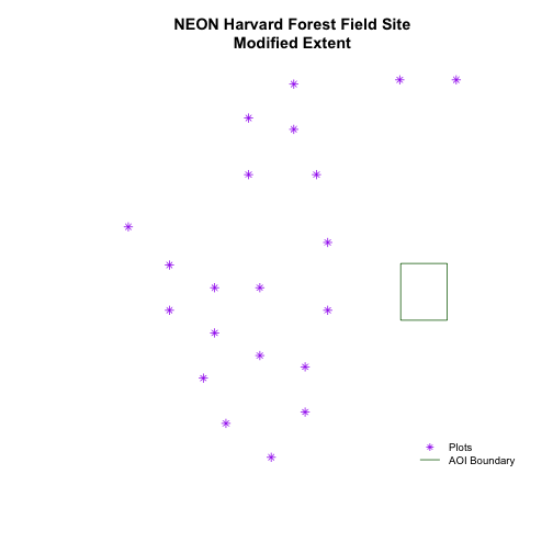
# adjust the plot extent using x and ylim
plot(aoiBoundary_HARV,
main="NEON Harvard Forest Field Site\nModified Extent",
border="darkgreen",
xlim=c(xmin,xmax),
ylim=c(ymin,ymax))
plot(plot.locationsSp_HARV,
pch=8,
col="purple",
add=TRUE)
# add a legend
legend("bottomright",
legend=c("Plots", "AOI Boundary"),
pch=c(8,NA),
lty=c(NA,1),
bty="n",
col=c("purple","darkgreen"),
cex=.8)
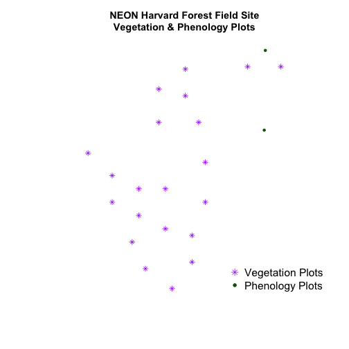
Import the .csv: HARV/HARV_2NewPhenPlots.csv into R and do the following:
- Find the X and Y coordinate locations. Which value is X and which value is Y?
- These data were collected in a geographic coordinate system (WGS84). Convert
the
data.frameinto an RspatialPointsDataFrame. - Plot the new points with the plot location points from above. Be sure to add a legend. Use a different symbol for the 2 new points! You may need to adjust the X and Y limits of your plot to ensure that both points are rendered by R!
If you have extra time, feel free to add roads and other layers to your map!
HINT: Refer to When Vector Data Don't Line Up - Handling Spatial Projection & CRS in R tutorial for more on working with geographic coordinate systems. You may want to "borrow" the projection from the objects used in that tutorial!
Export a Shapefile
We can write an R spatial object to a shapefile using the writeOGR function
in rgdal. To do this we need the following arguments:
- the name of the spatial object (
plot.locationsSp_HARV) - the directory where we want to save our shapefile
(to use
current = getwd()or you can specify a different path) - the name of the new shapefile (
PlotLocations_HARV) - the driver which specifies the file format (ESRI Shapefile)
We can now export the spatial object as a shapefile.
# write a shapefile
writeOGR(plot.locationsSp_HARV, getwd(),
         "PlotLocations_HARV", driver="ESRI Shapefile")