AGÕæÈË°Ù¼ÒÀÖ¹Ù·½ÍøÕ¾

This tutorial explores how to import and plot a multiband raster in R. It also covers how to plot a three-band color image using the plotRGB() function in R.

The Basics of Imagery - AGÕæÈË°Ù¼ÒÀÖ¹Ù·½ÍøÕ¾ Spectral Remote Sensing Data

AGÕæÈË°Ù¼ÒÀÖ¹Ù·½ÍøÕ¾ Raster Bands in R

As discussed in the Intro to Raster Data tutorial, a raster can contain 1 or more bands.

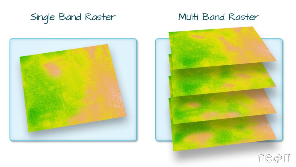
To work with multiband rasters in R, we need to change how we import and plot our data in several ways.

• To import multiband raster data we will use the stack() function.
• If our multiband data are imagery that we wish to composite, we can use plotRGB() (instead of plot()) to plot a 3 band raster image.

AGÕæÈË°Ù¼ÒÀÖ¹Ù·½ÍøÕ¾ MultiBand Imagery

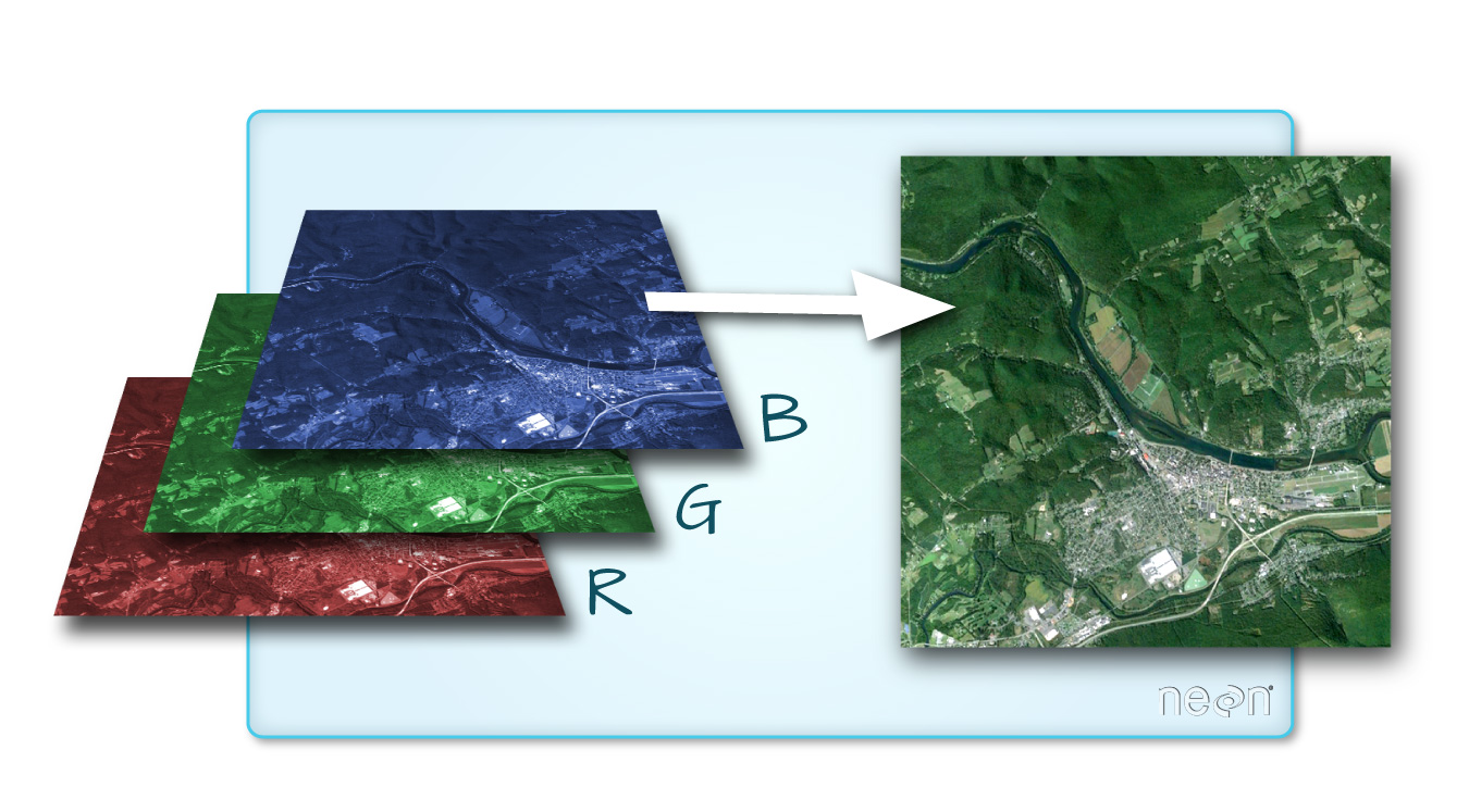
One type of multiband raster dataset that is familiar to many of us is a color image. A basic color image consists of three bands: red, green, and blue. Each band represents light reflected from the red, green or blue portions of the electromagnetic spectrum. The pixel brightness for each band, when composited creates the colors that we see in an image.

Getting Started with Multi-Band Data in R

To work with multiband raster data we will use the terra package.

# terra package to work with raster data

library(terra)



# package for downloading NEON data

library(neonUtilities)



# package for specifying color palettes

library(RColorBrewer)



# set working directory to ensure R can find the file we wish to import

wd <- "~/data/" # this will depend on your local environment environment

# be sure that the downloaded file is in this directory

setwd(wd)

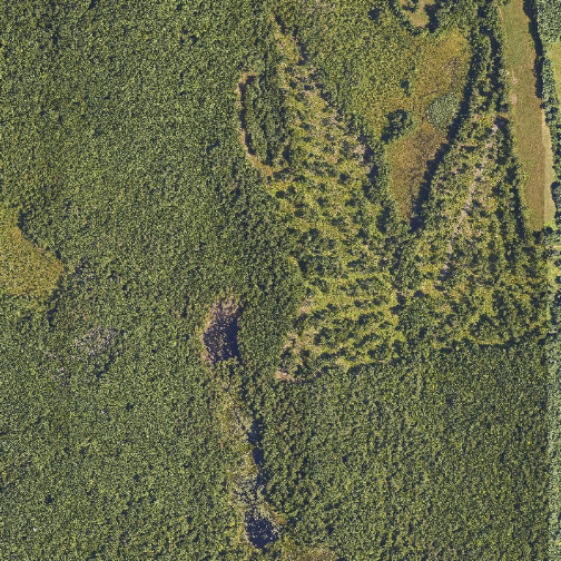
In this tutorial, the multi-band data that we are working with is imagery collected using the NEON Airborne Observation Platform high resolution camera over the NEON Harvard Forest field site. Each RGB image is a 3-band raster. The same steps would apply to working with a multi-spectral image with 4 or more bands - like Landsat imagery, or even hyperspectral imagery (in geotiff format). We can plot each band of a multi-band image individually.

byTileAOP(dpID='DP3.30010.001', # rgb camera data
          site='HARV',
          year='2022',
          easting=732000,
          northing=4713500,
          check.size=FALSE, # set to TRUE or remove if you want to check the size before downloading
          savepath = wd)

## Downloading files totaling approximately 351.004249 MB 
## Downloading 1 files
## 

|
| | 0% |
|====================================================================================================================================================================| 100% ## Successfully downloaded 1 files to ~/data//DP3.30010.001

Or we can plot each bands separately as follows:

# Determine the number of bands

num_bands <- nlyr(RGB_HARV)



# Define colors to plot each

# Define color palettes for each band using RColorBrewer

colors <- list(
  brewer.pal(9, "Reds"),
  brewer.pal(9, "Greens"),
  brewer.pal(9, "Blues")
)



# Plot each band in a loop, with the specified colors

for (i in 1:num_bands) {
  plot(RGB_HARV[[i]], main=paste("Band", i), col=colors[[i]])
}

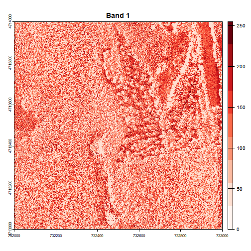
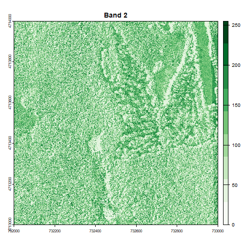
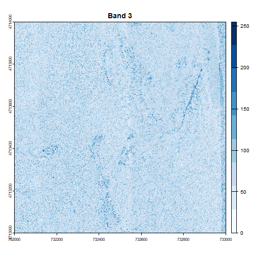
Image Raster Data Attributes

We can display some of the attributes about the raster, as shown below:

# Print dimensions

cat("Dimensions:\n")

## Dimensions:

cat("Number of rows:", nrow(RGB_HARV), "\n")

## Number of rows: 10000

cat("Number of columns:", ncol(RGB_HARV), "\n")

## Number of columns: 10000

cat("Number of layers:", nlyr(RGB_HARV), "\n")

## Number of layers: 3

# Print resolution

resolutions <- res(RGB_HARV)

cat("Resolution:\n")

## Resolution:

cat("X resolution:", resolutions[1], "\n")

## X resolution: 0.1

cat("Y resolution:", resolutions[2], "\n")

## Y resolution: 0.1

# Get the extent of the raster

rgb_extent <- ext(RGB_HARV)



# Convert the extent to a string with rounded values

extent_str <- sprintf("xmin: %d, xmax: %d, ymin: %d, ymax: %d", 
                      round(xmin(rgb_extent)), 
                      round(xmax(rgb_extent)), 
                      round(ymin(rgb_extent)), 
                      round(ymax(rgb_extent)))



# Print the extent string

cat("Extent of the raster: \n")

## Extent of the raster:

cat(extent_str, "\n")

## xmin: 732000, xmax: 733000, ymin: 4713000, ymax: 4714000

Let's take a look at the coordinate reference system, or CRS. You can use the parameters describe=TRUE to display this information more succinctly.

crs(RGB_HARV, describe=TRUE)

##                    name authority  code
## 1 WGS 84 / UTM zone 18N      EPSG 32618
##                                                                                                                                                                                                                                                          area
## 1 Between 78°W and 72°W, northern hemisphere between equator and 84°N, onshore and offshore. Bahamas. Canada - Nunavut; Ontario; Quebec. Colombia. Cuba. Ecuador. Greenland. Haiti. Jamaica. Panama. Turks and Caicos Islands. United States (USA). Venezuela
##            extent
## 1 -78, -72, 84, 0

Let's next examine the raster's minimum and maximum values. What is the range of values for each band?

# Replace Inf and -Inf with NA

values(RGB_HARV)[is.infinite(values(RGB_HARV))] <- NA



# Get min and max values for all bands

min_max_values <- minmax(RGB_HARV)



# Print the results

cat("Min and Max Values for All Bands:\n")

## Min and Max Values for All Bands:

print(min_max_values)

##     2022_HARV_7_732000_4713000_image_1 2022_HARV_7_732000_4713000_image_2 2022_HARV_7_732000_4713000_image_3
## min                                  0                                  0                                  0
## max                                255                                255                                255

This raster contains values between 0 and 255. These values represent the intensity of brightness associated with the image band. In the case of a RGB image (red, green and blue), band 1 is the red band. When we plot the red band, larger numbers (towards 255) represent pixels with more red in them (a strong red reflection). Smaller numbers (towards 0) represent pixels with less red in them (less red was reflected). To plot an RGB image, we mix red + green + blue values into one single color to create a full color image - this is the standard color image a digital camera creates.

Other Types of Multi-band Raster Data

Multi-band raster data might also contain:

1. Time series: the same variable, over the same area, over time.
2. Multi or hyperspectral imagery: image rasters that have 4 or more (multi-spectral) or more than 10-15 (hyperspectral) bands. Check out the NEON Data Skills Imaging Spectroscopy HDF5 in R tutorial to learn how to work with hyperspectral data cubes.

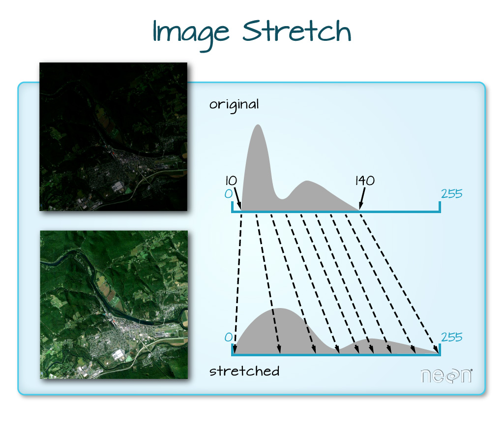
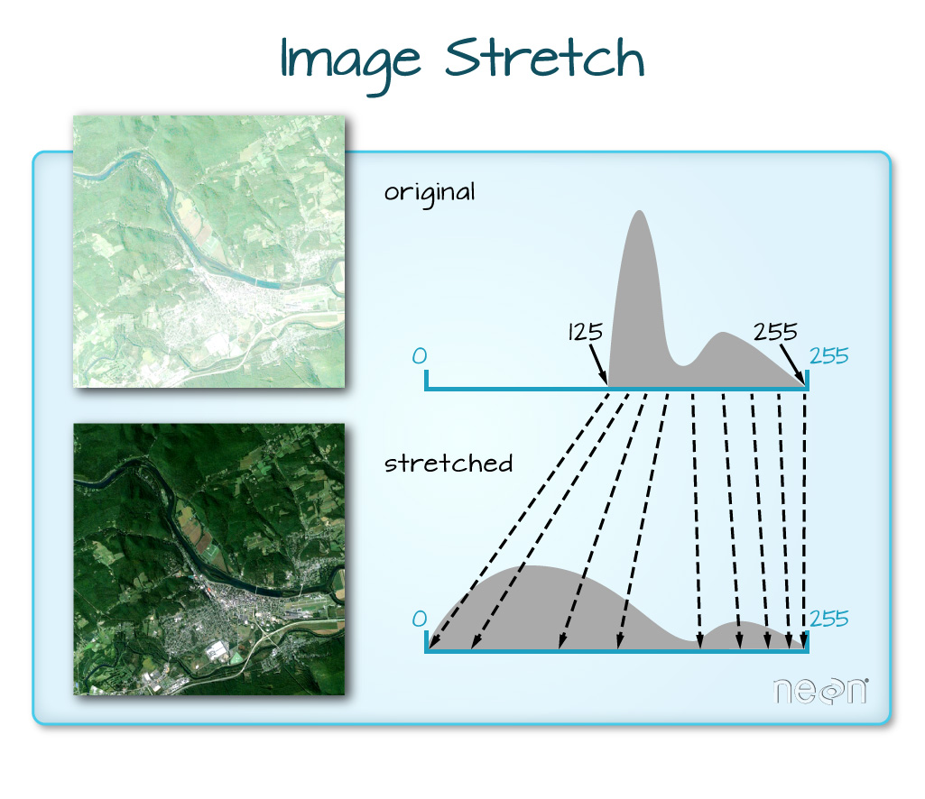
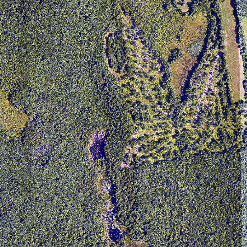
The true color image plotted at the beginning of this lesson looks pretty decent. We can explore whether applying a stretch to the image might improve clarity and contrast using stretch="lin" or stretch="hist".

# What does stretch do?



# Plot the linearly stretched raster

plotRGB(RGB_HARV, stretch="lin")

# Plot the histogram-stretched raster

plotRGB(RGB_HARV, stretch="hist")

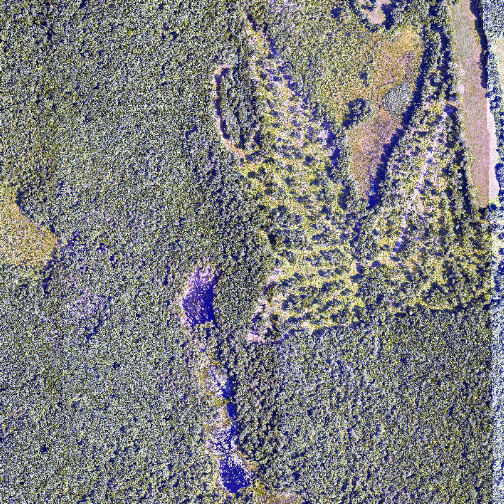
In this case, the stretch doesn't enhance the contrast our image significantly given the distribution of reflectance (or brightness) values is distributed well between 0 and 255, and applying a stretch appears to introduce some artificial, almost purple-looking brightness to the image.