Tutorial
Vector 00: Open and Plot Shapefiles in R - Getting Started with Point, Line and Polygon Vector Data
Last Updated: Apr 8, 2021
In this tutorial, we will open and plot point, line and polygon vector data stored in shapefile format in R.
Learning Objectives
After completing this tutorial, you will be able to:
- Explain the difference between point, line, and polygon vector elements.
- Describe the differences between opening point, line and polygon shapefiles in R.
- Describe the components of a spatial object in R.
- Read a shapefile into R.
Things You’ll Need To Complete This Tutorial
You will need the most current version of R and, preferably, RStudio loaded
on your computer to complete this tutorial.
Install R Packages
-
raster:
install.packages("raster") -
rgdal:
install.packages("rgdal") -
sp:
install.packages("sp")
More on Packages in R � Adapted from Software Carpentry.
Download Data
These vector data provide information on the site characterization and infrastructure at the National Ecological Observatory Network's Harvard Forest field site. The Harvard Forest shapefiles are from the archives. US Country and State Boundary layers are from the .
Set Working Directory: This lesson assumes that you have set your working directory to the location of the downloaded and unzipped data subsets.
An overview of setting the working directory in R can be found here.
R Script & Challenge Code: NEON data lessons often contain challenges that reinforce learned skills. If available, the code for challenge solutions is found in the downloadable R script of the entire lesson, available in the footer of each lesson page.
AGŐćČË°ŮĽŇŔֹٷ˝ÍřŐľ Vector Data
Vector data are composed of discrete geometric locations (x,y values) known as vertices that define the "shape" of the spatial object. The organization of the vertices, determines the type of vector that we are working with: point, line or polygon.
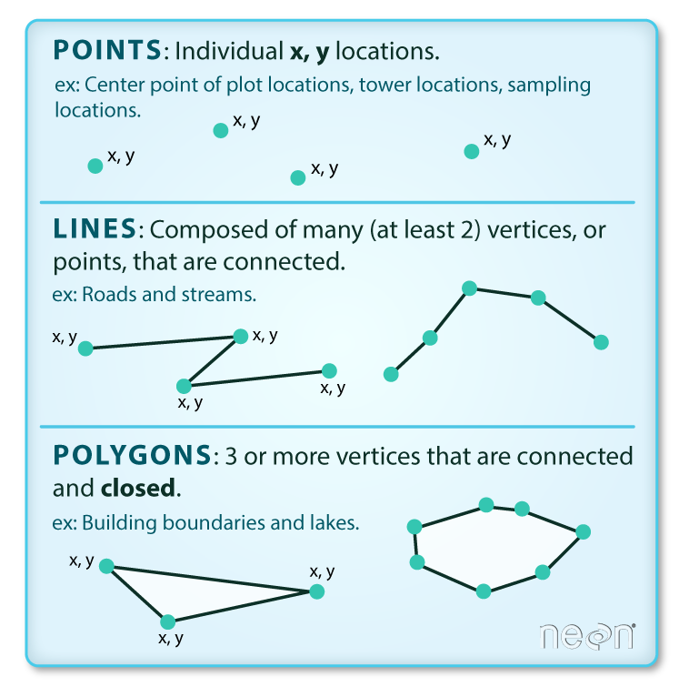
- Points: Each individual point is defined by a single x, y coordinate. There can be many points in a vector point file. Examples of point data include: sampling locations, the location of individual trees or the location of plots.
-
Lines: Lines are composed of many (at least 2) vertices, or points, that
are connected. For instance, a road or a stream may be represented by a line. This
line is composed of a series of segments, each "bend" in the road or stream
represents a vertex that has defined
x, ylocation. - Polygons: A polygon consists of 3 or more vertices that are connected and "closed". Thus the outlines of plot boundaries, lakes, oceans, and states or countries are often represented by polygons. Occasionally, a polygon can have a hole in the middle of it (like a doughnut), this is something to be aware of but not an issue we will deal with in this tutorial.
Shapefiles: Points, Lines, and Polygons
Geospatial data in vector format are often stored in a shapefile format.
Because the structure of points, lines, and polygons are different, each
individual shapefile can only contain one vector type (all points, all lines
or all polygons). You will not find a mixture of point, line and polygon
objects in a single shapefile.
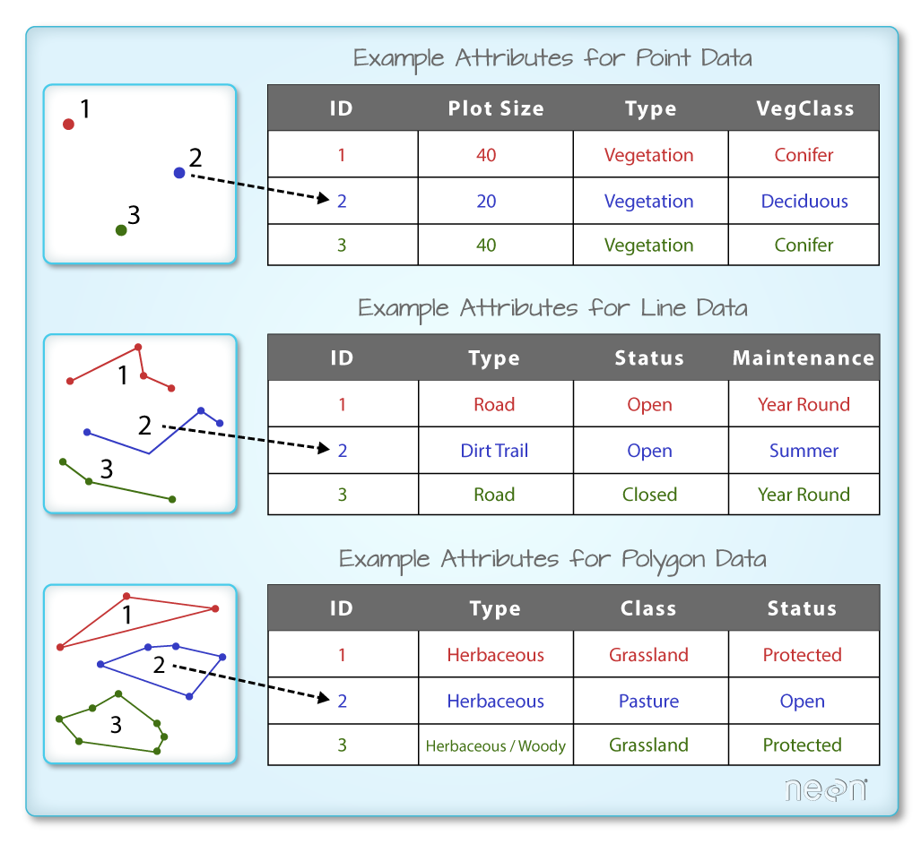
Objects stored in a shapefile often have a set of associated attributes that
describe the data. For example, a line shapefile that contains the locations of
streams, might contain the associated stream name, stream "order" and other
information about each stream line object.
- More about shapefiles can found on .
Import Shapefiles
We will use the rgdal package to work with vector data in R. Notice that the
sp package automatically loads when rgdal is loaded. We will also load the
raster package so we can explore raster and vector spatial metadata using similar commands.
# load required libraries
# for vector work; sp package will load with rgdal.
library(rgdal)
# for metadata/attributes- vectors or rasters
library(raster)

# set working directory to the directory location on your computer where
# you downloaded and unzipped the data files for the tutorial
# setwd("pathToDirHere")
The shapefiles that we will import are:
- A polygon shapefile representing our field site boundary,
- A line shapefile representing roads, and
- A point shapefile representing the location of the Fisher
flux tower located at the NEON Harvard Forest field site.
The first shapefile that we will open contains the boundary of our study area
(or our Area Of Interest or AOI, hence the name aoiBoundary). To import
shapefiles we use the R function readOGR().
readOGR() requires two components:
- The directory where our shapefile lives:
NEON-DS-Site-Layout-Files/HARV - The name of the shapefile (without the extension):
HarClip_UTMZ18
Let's import our AOI.
# Import a polygon shapefile: readOGR("path","fileName")
# no extension needed as readOGR only imports shapefiles
aoiBoundary_HARV <- readOGR(dsn=path.expand("NEON-DS-Site-Layout-Files/HARV"),
                            layer="HarClip_UTMZ18")

## OGR data source with driver: ESRI Shapefile
## Source: "/Users/olearyd/Git/data/NEON-DS-Site-Layout-Files/HARV", layer: "HarClip_UTMZ18"
## with 1 features
## It has 1 fields
## Integer64 fields read as strings:  id
Shapefile Metadata & Attributes
When we import the HarClip_UTMZ18 shapefile layer into R (as our
aoiBoundary_HARV object), the readOGR() function automatically stores
information about the data. We are particularly interested in the geospatial
metadata, describing the format, CRS, extent, and other components of
the vector data, and the attributes which describe properties associated
with each individual vector object.
Spatial Metadata
Key metadata for all shapefiles include:
- Object Type: the class of the imported object.
- Coordinate Reference System (CRS): the projection of the data.
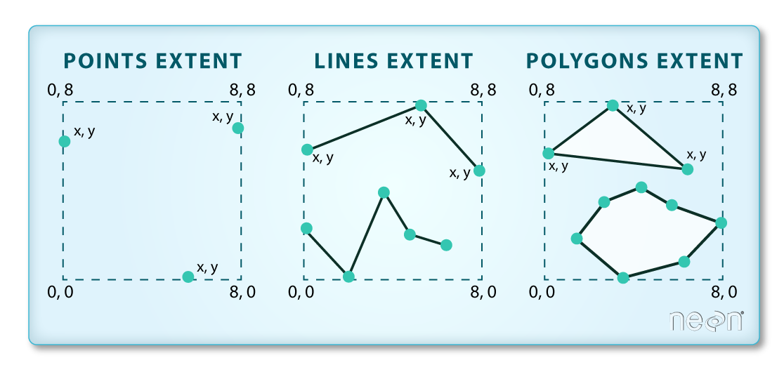
- Extent: the spatial extent (geographic area that the shapefile covers) of the shapefile. Note that the spatial extent for a shapefile represents the extent for ALL spatial objects in the shapefile.
We can view shapefile metadata using the class, crs and extent methods:
# view just the class for the shapefile
class(aoiBoundary_HARV)

## [1] "SpatialPolygonsDataFrame"
## attr(,"package")
## [1] "sp"

# view just the crs for the shapefile
crs(aoiBoundary_HARV)

## CRS arguments:
##  +proj=utm +zone=18 +datum=WGS84 +units=m +no_defs

# view just the extent for the shapefile
extent(aoiBoundary_HARV)

## class      : Extent
## xmin       : 732128
## xmax       : 732251.1
## ymin       : 4713209
## ymax       : 4713359

# view all metadata at same time
aoiBoundary_HARV

## class       : SpatialPolygonsDataFrame
## features    : 1
## extent      : 732128, 732251.1, 4713209, 4713359  (xmin, xmax, ymin, ymax)
## crs         : +proj=utm +zone=18 +datum=WGS84 +units=m +no_defs
## variables   : 1
## names       : id
## value       :  1
Our aoiBoundary_HARV object is a polygon of class SpatialPolygonsDataFrame,
in the CRS UTM zone 18N. The CRS is critical to interpreting the object
extent values as it specifies units.
Spatial Data Attributes
Each object in a shapefile has one or more attributes associated with it. Shapefile attributes are similar to fields or columns in a spreadsheet. Each row in the spreadsheet has a set of columns associated with it that describe the row element. In the case of a shapefile, each row represents a spatial object - for example, a road, represented as a line in a line shapefile, will have one "row" of attributes associated with it. These attributes can include different types of information that describe objects stored within a shapefile. Thus, our road, may have a name, length, number of lanes, speed limit, type of road and other attributes stored with it.
We view the attributes of a SpatialPolygonsDataFrame using objectName@data
(e.g., aoiBoundary_HARV@data).
# alternate way to view attributes
aoiBoundary_HARV@data

##   id
## 0  1
In this case, our polygon object only has one attribute: id.
Metadata & Attribute Summary
We can view a metadata & attribute summary of each shapefile by entering
the name of the R object in the console. Note that the metadata output
includes the class, the number of features, the extent, and the
coordinate reference system (crs) of the R object. The last two lines of
summary show a preview of the R object attributes.
# view a summary of metadata & attributes associated with the spatial object
summary(aoiBoundary_HARV)

## Object of class SpatialPolygonsDataFrame
## Coordinates:
##       min       max
## x  732128  732251.1
## y 4713209 4713359.2
## Is projected: TRUE
## proj4string :
## [+proj=utm +zone=18 +datum=WGS84 +units=m +no_defs]
## Data attributes:
##       id
##  Length:1
##  Class :character
##  Mode  :character
Plot a Shapefile
Next, let's visualize the data in our R spatialpolygonsdataframe object using
plot().
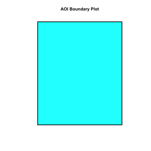
# create a plot of the shapefile
# 'lwd' sets the line width
# 'col' sets internal color
# 'border' sets line color
plot(aoiBoundary_HARV, col="cyan1", border="black", lwd=3,
     main="AOI Boundary Plot")
Answer the following questions:
- What type of R spatial object is created when you import each layer?
- What is the
CRSandextentfor each object? - Do the files contain, points, lines or polygons?
- How many spatial objects are in each file?
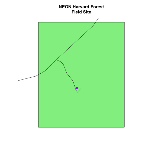
Plot Multiple Shapefiles
The plot() function can be used for basic plotting of spatial objects.
We use the add = TRUE argument to overlay shapefiles on top of each other, as
we would when creating a map in a typical GIS application like QGIS.
We can use main="" to give our plot a title. If we want the title to span two
lines, we use \n where the line should break.
# Plot multiple shapefiles
plot(aoiBoundary_HARV, col = "lightgreen",
     main="NEON Harvard Forest\nField Site")
plot(lines_HARV, add = TRUE)

# use the pch element to adjust the symbology of the points
plot(point_HARV, add  = TRUE, pch = 19, col = "purple")
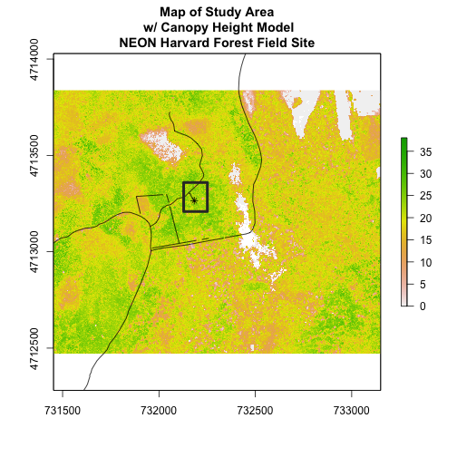
You can plot vector data layered on top of raster data using the add=TRUE
plot attribute. Create a plot that uses the NEON AOP Canopy Height Model NEON_RemoteSensing/HARV/CHM/HARV_chmCrop.tif as a base layer. On top of the
CHM, please add:
- The study site AOI.
- Roads.
- The tower location.
Be sure to give your plot a meaningful title.
For assistance consider using the Shapefile Metadata & Attributes in R and the Plot Raster Data in R tutorials.
Additional Resources: Plot Parameter Options
For more on parameter options in the base R plot() function, check out these
resources: