Tutorial
Time Series 03: Cleaning & Subsetting Time Series Data in R - NoData Values & Subset by Date
Last Updated: May 13, 2021
This tutorial explores how to deal with NoData values encountered in a time
series dataset, in R. It also covers how to subset large files by date and
export the results to a .csv (text) file.
Learning Objectives
After completing this tutorial, you will be able to:
- Subset data by date.
- Search for NA or missing data values.
- Describe different possibilities on how to deal with missing data.
Things You’ll Need To Complete This Tutorial
You will need the most current version of R and, preferably, RStudio loaded on your computer to complete this tutorial.
Install R Packages
-
lubridate:
install.packages("lubridate") -
ggplot2:
install.packages("ggplot2")
More on Packages in R � Adapted from Software Carpentry.
Download Data
The data used in this lesson were collected at the National Ecological Observatory Network's Harvard Forest field site. These data are proxy data for what will be available for 30 years on the for the Harvard Forest and other field sites located across the United States.
Set Working Directory: This lesson assumes that you have set your working directory to the location of the downloaded and unzipped data subsets.
An overview of setting the working directory in R can be found here.
R Script & Challenge Code: NEON data lessons often contain challenges that reinforce learned skills. If available, the code for challenge solutions is found in the downloadable R script of the entire lesson, available in the footer of each lesson page.
Cleaning Time Series Data
It is common to encounter, large files containing more
data than we need for our analysis. It is also common to encounter NoData
values that we need to account for when analyzing our data.
In this tutorial, we'll learn how to both manage NoData values and also
subset and export a portion of an R object as a new .csv file.
In this tutorial, we will work with atmospheric data, containing air temperature, precipitation, and photosynthetically active radiation (PAR) data - metrics that are key drivers of phenology. Our study area is the NEON Harvard Forest Field Site.
Import Timeseries Data
We will use the lubridate and ggplot2 packages. Let's load those first.
If you have not already done so, import the hf001-10-15min-m.csv file, which
contains atmospheric data for Harvard Forest. Convert the datetime column
to a POSIXct class as covered in the tutorial:
Dealing With Dates & Times in R - as.Date, POSIXct, POSIXlt.
# Load packages required for entire script
library(lubridate)  # work with dates
library(ggplot2)  # plotting

# set working directory to ensure R can find the file we wish to import
wd <- "~/Git/data/"

# Load csv file containing 15 minute averaged atmospheric data
# for the NEON Harvard Forest Field Site

# Factors=FALSE so data are imported as numbers and characters
harMet_15Min <- read.csv(
  file=paste0(wd,"NEON-DS-Met-Time-Series/HARV/FisherTower-Met/hf001-10-15min-m.csv"),
  stringsAsFactors = FALSE)

# convert to POSIX date time class - US Eastern Time Zone
harMet_15Min$datetime <- as.POSIXct(harMet_15Min$datetime,
                                format = "%Y-%m-%dT%H:%M",
                                tz = "America/New_York")
Subset by Date
Our .csv file contains nearly a decade's worth of data which makes for a large
file. The time period we are interested in for our study is:
- Start Time: 1 January 2009
- End Time: 31 Dec 2011
Let's subset the data to only contain these three years. We can use the
subset() function, with the syntax:
NewObject <- subset ( ObjectToBeSubset, CriteriaForSubsetting ) .
We will set our criteria to be any datetime that:
- Is greater than or equal to 1 Jan 2009 at 0:00 AND
- Is less than or equal to 31 Dec 2011 at 23:59.
We also need to specify the timezone so R can handle daylight savings and
leap year.
# subset data - 2009-2011
harMet15.09.11 <- subset(harMet_15Min,
                         datetime >= as.POSIXct('2009-01-01 00:00',
                                                tz = "America/New_York") &
                         datetime <= as.POSIXct('2011-12-31 23:59',
                                               tz = "America/New_York"))

# View first and last records in the object
head(harMet15.09.11[1])

##                   datetime
## 140255 2009-01-01 00:00:00
## 140256 2009-01-01 00:15:00
## 140257 2009-01-01 00:30:00
## 140258 2009-01-01 00:45:00
## 140259 2009-01-01 01:00:00
## 140260 2009-01-01 01:15:00

tail(harMet15.09.11[1])

##                   datetime
## 245369 2011-12-31 22:30:00
## 245370 2011-12-31 22:45:00
## 245371 2011-12-31 23:00:00
## 245372 2011-12-31 23:15:00
## 245373 2011-12-31 23:30:00
## 245374 2011-12-31 23:45:00
It worked! The first entry is 1 January 2009 at 00:00 and the last entry is 31 December 2011 at 23:45.
Export data.frame to .CSV
We can export this subset in .csv format to use in other analyses or to
share with colleagues using write.csv.
# write harMet15 subset data to .csv
write.csv(harMet15.09.11,
          file=paste0(wd,"Met_HARV_15min_2009_2011.csv"))
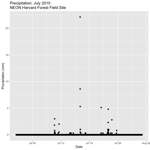
-
Create a plot of precipitation for the month of July 2010 in Harvard Forest. Be sure to label x and y axes. Also be sure to give your plot a title.
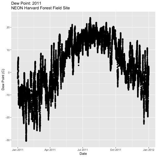
-
Create a plot of dew point (
dewp) for the year 2011 at Harvard Forest.
Bonus challenge: Complete this challenge using the available daily data instead of the 15-minute data. What will need to change in your subsetting code?
Managing Missing Data: NoData values
Find NoData Values
If we are lucky when working with external data, the NoData value is clearly
specified
in the metadata. No data values can be stored differently:
-
NA / NaN: Sometimes this value is
NAorNaN(not a number). -
A Designated Numeric Value (e.g. -9999): Character strings such as
NAcan not always be stored along side of numeric values in some file formats. Sometimes you'll encounter numeric placeholders fornoDatavalues such as-9999(a value often used in the GIS / Remote Sensing and Micrometeorology domains. -
Blank Values: sometimes
noDatavalues are left blank. Blanks are particularly problematic because we can't be certain if a data value is purposefully missing (not measured that day or a bad measurement) or if someone unintentionally deleted it.
Because the actual value used to designate missing data can vary depending upon
what data we are working with, it is important to always check the metadata for
the files associated NoData value. If the value is NA, we are in luck, R
will recognize and flag this value as NoData. If the value is numeric (e.g.,
-9999), then we might need to assign this value to NA.
In the
Why Metadata Are Important: How to Work with Metadata in Text & EML Format tutorial,
we viewed the metadata for these data and discovered that missing values are
designated using NA - a common NoData value placeholder.
Excerpt from the metadata:
airt: average air temperature. Average of daily averages. (unit: celsius / missing value: NA)
Check For NoData Values
We can quickly check for NoData values in our data using theis.na()
function. By asking for the sum() of is.na() we can see how many NA/ missing
values we have.
# Check for NA values
sum(is.na(harMet15.09.11$datetime))

## [1] 0

sum(is.na(harMet15.09.11$airt))

## [1] 2

# view rows where the air temperature is NA
harMet15.09.11[is.na(harMet15.09.11$airt),]

##                   datetime  jd airt f.airt rh f.rh dewp f.dewp prec
## 158360 2009-07-08 14:15:00 189   NA      M NA    M   NA      M    0
## 203173 2010-10-18 09:30:00 291   NA      M NA    M   NA      M    0
##        f.prec slrr f.slrr parr f.parr netr f.netr bar f.bar wspd
## 158360         290         485         139         NA     M  2.1
## 203173          NA      M   NA      M   NA      M  NA     M   NA
##        f.wspd wres f.wres wdir f.wdir wdev f.wdev gspd f.gspd s10t
## 158360         1.8          86          29         5.2        20.7
## 203173      M   NA      M   NA      M   NA      M   NA      M 10.9
##        f.s10t
## 158360
## 203173
The results above tell us there are NoData values in the airt column.
However, there are NoData values in other variables.
How many NoData values are in the precipitation (prec) and PAR (parr)
columns of our data?
Deal with NoData Values
When we encounter NoData values (blank, NaN, -9999, etc.) in our data we
need to decide how to deal with them. By default R treats NoData values
designated with a NA as a missing value rather than a zero. This is good, as a
value of zero (no rain today) is not the same as missing data (e.g. we didn't
measure the amount of rainfall today).
How we deal with NoData values will depend on:
- the data type we are working with
- the analysis we are conducting
- the significance of the gap or missing value
Many functions in R contains a na.rm= option which will allow you to tell R
to ignore NA values in your data when performing calculations.
To Gap Fill? Or Not?
Sometimes we might need to "gap fill" our data. This means we will interpolate or estimate missing values often using statistical methods. Gap filling can be complex and is beyond the scope of this tutorial. The take away from this is simply that it is important to acknowledge missing values in your data and to carefully consider how you wish to account for them during analysis.
Other resources:
- R code for dealing with missing data:
Managing NoData Values in Our Data
For this tutorial, we are exploring the patterns of precipitation,
and temperature as they relate to green-up and brown-down of vegetation at
Harvard Forest. To view overall trends during these early exploration stages, it
is okay for us to leave out the NoData values in our plots.
NoData Values Can Impact Calculations
It is important to consider NoData values when performing calculations on our
data. For example, R will not properly calculate certain functions if there
are NA values in the data, unless we explicitly tell it to ignore them.
# calculate mean of air temperature
mean(harMet15.09.11$airt)

## [1] NA

# are there NA values in our data?
sum(is.na(harMet15.09.11$airt))

## [1] 2
R will not return a value for the mean as there NA values in the air
temperature column. Because there are only 2 missing values (out of 105,108) for
air temperature, we aren't that worried about a skewed 3 year mean. We can tell
R to ignore noData values in the mean calculations using na.rm=
(NA.remove).
# calculate mean of air temperature, ignore NA values
mean(harMet15.09.11$airt,
     na.rm=TRUE)

## [1] 8.467904
We now see that the 3-year average air temperature is 8.5°C.
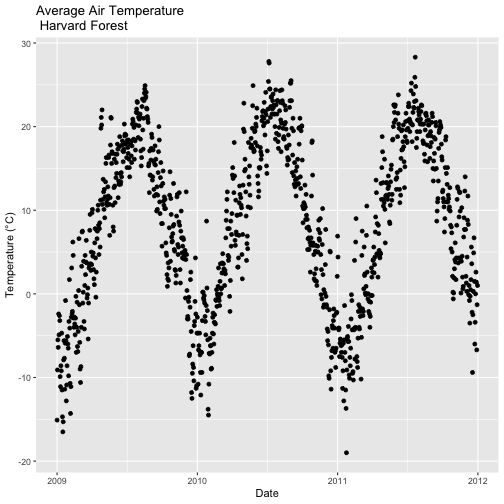
- Import the Daily Meteorological data from the Harvard Forest (if you haven't already done so in the Intro to Time Series Data in R tutorial.)
- Check the metadata to see what the column names are for the variable of interest (precipitation, air temperature, PAR, day and time ).
- If needed, convert the data class of different columns.
- Check for missing data and decide what to do with any that exist.
- Subset out the data for the duration of our study: 2009-2011. Name the object "harMetDaily.09.11".
- Export the subset to a
.csvfile. - Create a plot of Daily Air Temperature for 2009-2011. Be sure to label, x- and y-axes. Also give the plot a title!