Tutorial
Time Series 04: Subset and Manipulate Time Series Data with dplyr
Last Updated: May 13, 2021
In this tutorial, we will use the group_by, summarize and mutate functions
in the dplyr package to efficiently manipulate atmospheric data collected at
the NEON Harvard Forest Field Site. We will use pipes to efficiently perform
multiple tasks within a single chunk of code.
Learning Objectives
After completing this tutorial, you will be able to:
- Explain several ways to manipulate data using functions in the
dplyrpackage in R. - Use
group-by(),summarize(), andmutate()functions. - Write and understand R code with pipes for cleaner, efficient coding.
- Use the
year()function from thelubridatepackage to extract year from a date-time class variable.
Things You’ll Need To Complete This Tutorial
You will need the most current version of R and, preferably, RStudio loaded on your computer to complete this tutorial.
Install R Packages
-
lubridate:
install.packages("lubridate") -
dplyr:
install.packages("dplyr") -
ggplot2:
install.packages("ggplot2")
More on Packages in R � Adapted from Software Carpentry.
Download Data
The data used in this lesson were collected at the National Ecological Observatory Network's Harvard Forest field site. These data are proxy data for what will be available for 30 years on the for the Harvard Forest and other field sites located across the United States.
Set Working Directory: This lesson assumes that you have set your working directory to the location of the downloaded and unzipped data subsets.
An overview of setting the working directory in R can be found here.
R Script & Challenge Code: NEON data lessons often contain challenges that reinforce learned skills. If available, the code for challenge solutions is found in the downloadable R script of the entire lesson, available in the footer of each lesson page.
Additional Resources
- NEON Data Skills tutorial on spatial data and piping with dplyr
- Data Carpentry lesson's on
- .
Introduction to dplyr
The dplyr package simplifies and increases efficiency of complicated yet
commonly performed data "wrangling" (manipulation / processing) tasks. It uses
the data_frame object as both an input and an output.
Load the Data
We will need the lubridate and the dplyr packages to complete this tutorial.
We will also use the 15-minute average atmospheric data subsetted to 2009-2011 for the NEON Harvard Forest Field Site. This subset was created in the Subsetting Time Series Data tutorial.
If this object isn't already created, please load the .csv version:
Met_HARV_15min_2009_2011.csv. Be
sure to convert the date-time column to a POSIXct class after the .csv is
loaded.
# it's good coding practice to load packages at the top of a script

library(lubridate) # work with dates
library(dplyr)     # data manipulation (filter, summarize, mutate)
library(ggplot2)   # graphics
library(gridExtra) # tile several plots next to each other
library(scales)

# set working directory to ensure R can find the file we wish to import
wd <- "~/Git/data/"

# 15-min Harvard Forest met data, 2009-2011
harMet15.09.11<- read.csv(
  file=paste0(wd,"NEON-DS-Met-Time-Series/HARV/FisherTower-Met/Met_HARV_15min_2009_2011.csv"),
  stringsAsFactors = FALSE)

# convert datetime to POSIXct
harMet15.09.11$datetime<-as.POSIXct(harMet15.09.11$datetime,
                    format = "%Y-%m-%d %H:%M",
                    tz = "America/New_York")
Explore The Data
Remember that we are interested in the drivers of phenology including - air temperature, precipitation, and PAR (photosynthetic active radiation - or the amount of visible light). Using the 15-minute averaged data, we could easily plot each of these variables.
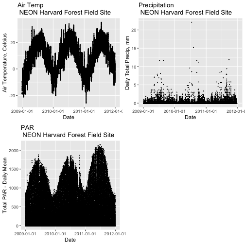
However, summarizing the data at a coarser scale (e.g., daily, weekly, by season, or by year) may be easier to visually interpret during initial stages of data exploration.
Extract Year from a Date-Time Column
To summarize by year efficiently, it is helpful to have a year column that we
can use to group by. We can use the lubridate function year() to extract
the year only from a date-time class R column.
# create a year column
harMet15.09.11$year <- year(harMet15.09.11$datetime)
Using names() we see that we now have a year column in our data_frame.
# check to make sure it worked
names(harMet15.09.11)

##  [1] "X"        "datetime" "jd"       "airt"     "f.airt"   "rh"
##  [7] "f.rh"     "dewp"     "f.dewp"   "prec"     "f.prec"   "slrr"
## [13] "f.slrr"   "parr"     "f.parr"   "netr"     "f.netr"   "bar"
## [19] "f.bar"    "wspd"     "f.wspd"   "wres"     "f.wres"   "wdir"
## [25] "f.wdir"   "wdev"     "f.wdev"   "gspd"     "f.gspd"   "s10t"
## [31] "f.s10t"   "year"

str(harMet15.09.11$year)

##  num [1:105108] 2009 2009 2009 2009 2009 ...
Now that we have added a year column to our data_frame, we can use dplyr to
summarize our data.
Manipulate Data using dplyr
Let's start by extracting a yearly air temperature value for the Harvard Forest data. To calculate a yearly average, we need to:
- Group our data by year.
- Calculate the mean precipitation value for each group (ie for each year).
We will use dplyr functions group_by and summarize to perform these steps.
# Create a group_by object using the year column
HARV.grp.year <- group_by(harMet15.09.11, # data_frame object
                          year) # column name to group by

# view class of the grouped object
class(HARV.grp.year)

## [1] "grouped_df" "tbl_df"     "tbl"        "data.frame"
The group_by function creates a "grouped" object. We can then use this
grouped object to quickly calculate summary statistics by group - in this case,
year. For example, we can count how many measurements were made each year using
the tally() function. We can then use the summarize function to calculate
the mean air temperature value each year. Note that "summarize" is a common
function name across many different packages. If you happen to have two packages
loaded at the same time that both have a "summarize" function, you may not get
the results that you expect. Therefore, we will "disambiguate" our function by
specifying which package it comes from using the double colon notation
dplyr::summarize().
# how many measurements were made each year?
tally(HARV.grp.year)

## # A tibble: 3 x 2
##    year     n
##   <dbl> <int>
## 1  2009 35036
## 2  2010 35036
## 3  2011 35036

# what is the mean airt value per year?
dplyr::summarize(HARV.grp.year,
          mean(airt)   # calculate the annual mean of airt
          )

## # A tibble: 3 x 2
##    year `mean(airt)`
##   <dbl>        <dbl>
## 1  2009        NA
## 2  2010        NA
## 3  2011         8.75
Why did this return a NA value for years 2009 and 2010? We know there are some
values for both years. Let's check our data for NoData values.
# are there NoData values?
sum(is.na(HARV.grp.year$airt))

## [1] 2

# where are the no data values
# just view the first 6 columns of data
HARV.grp.year[is.na(HARV.grp.year$airt),1:6]

## # A tibble: 2 x 6
##        X datetime               jd  airt f.airt    rh
##    <int> <dttm>              <int> <dbl> <chr>  <int>
## 1 158360 2009-07-08 14:15:00   189    NA M         NA
## 2 203173 2010-10-18 09:30:00   291    NA M         NA
It appears as if there are two NoData values (in 2009 and 2010) that are
causing R to return a NA for the mean for those years. As we learned
previously, we can use na.rm to tell R to ignore those values and calculate
the final mean value.
# calculate mean but remove NA values
dplyr::summarize(HARV.grp.year,
          mean(airt, na.rm = TRUE)
          )

## # A tibble: 3 x 2
##    year `mean(airt, na.rm = TRUE)`
##   <dbl>                      <dbl>
## 1  2009                       7.63
## 2  2010                       9.03
## 3  2011                       8.75
Great! We've now used the group_by function to create groups for each year
of our data. We then calculated a summary mean value per year using summarize.
dplyr Pipes
The above steps utilized several steps of R code and created 1 R object -
HARV.grp.year. We can combine these steps using pipes in the dplyr
package.
We can use pipes to string functions or processing steps together. The output
of each step is fed directly into the next step using the syntax: %>%. This
means we don't need to save the output of each intermediate step as a new R
object.
A few notes about piping syntax:
- A pipe begins with the object name that we will be manipulating, in our case
harMet15.09.11. - It then links that object with first manipulation step using
%>%. - Finally, the first function is called, in our case
group_by(year). Note that because we specified the object name in step one above, we can just use the column name
So, we have: harMet15.09.11 %>% group_by(year)
- We can then add an additional function (or more functions!) to our pipe. For
example, we can tell R to
tallyor count the number of measurements per year.
harMet15.09.11 %>% group_by(year) %>% tally()
Let's try it!
# how many measurements were made a year?
harMet15.09.11 %>%
  group_by(year) %>%  # group by year
  tally() # count measurements per year

## # A tibble: 3 x 2
##    year     n
##   <dbl> <int>
## 1  2009 35036
## 2  2010 35036
## 3  2011 35036
Piping allows us to efficiently perform operations on our data_frame in that:
- It allows us to condense our code, without naming intermediate steps.
- The dplyr package is optimized to ensure fast processing!
We can use pipes to summarize data by year too:
# what was the annual air temperature average
year.sum <- harMet15.09.11 %>%
group_by(year) %>% # group by year
dplyr::summarize(mean(airt, na.rm=TRUE))
# what is the class of the output?
year.sum
## # A tibble: 3 x 2
## year `mean(airt, na.rm = TRUE)`
## <dbl> <dbl>
## 1 2009 7.63
## 2 2010 9.03
## 3 2011 8.75
# view structure of output
str(year.sum)
## tibble [3 Ă— 2] (S3: tbl_df/tbl/data.frame)
## $ year : num [1:3] 2009 2010 2011
## $ mean(airt, na.rm = TRUE): num [1:3] 7.63 9.03 8.75
Other dplyr Functions
dplyr works based on a series of verb functions that allow us to manipulate
the data in different ways:
-
filter()&slice(): filter rows based on values in specified columns -
group-by(): group all data by a column -
arrange(): sort data by values in specified columns -
select()&rename(): view and work with data from only specified columns -
distinct(): view and work with only unique values from specified columns -
mutate()&transmute(): add new data to a data frame -
summarise(): calculate the specified summary statistics -
sample_n()&sample_frac(): return a random sample of rows
(List modified from the CRAN dplyr
. )
The syntax for all dplyr functions is similar:
- the first argument is the target
data_frame, - the subsequent arguments dictate what to do with that
data_frameand - the output is a new data frame.
Group by a Variable (or Two)
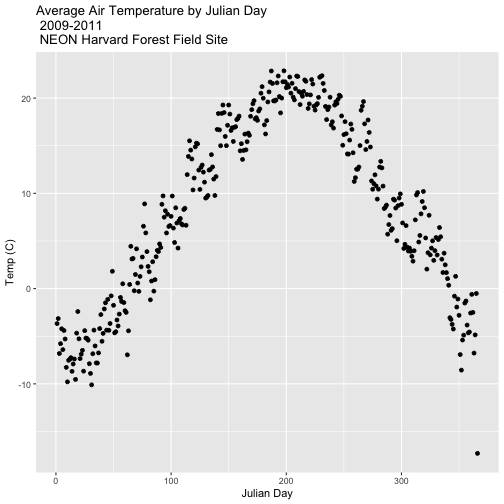
Our goal for this tutorial is to view drivers of annual phenology patterns.
Specifically, we want to explore daily average temperature throughout the year.
This means we need to calculate average temperature, for each day, across three
years. To do this we can use the group_by() function as we did earlier.
However this time, we can group by two variables: year and Julian Day (jd) as follows:
group_by(year, jd)
Let's begin by counting or tallying the total measurements per Julian day (or
year day) using the group_by() function and pipes.
harMet15.09.11 %>% # use the harMet15.09.11 data_frame
group_by(year, jd) %>% # group data by Year & Julian day
tally() # tally (count) observations per jd / year
## # A tibble: 1,096 x 3
## # Groups: year [3]
## year jd n
## <dbl> <int> <int>
## 1 2009 1 96
## 2 2009 2 96
## 3 2009 3 96
## 4 2009 4 96
## 5 2009 5 96
## 6 2009 6 96
## 7 2009 7 96
## 8 2009 8 96
## 9 2009 9 96
## 10 2009 10 96
## # � with 1,086 more rows
The output shows we have 96 values for each day. Is that what we expect?
24*4  # 24 hours/day * 4 15-min data points/hour

## [1] 96
Summarize by Group
We can use summarize() function to calculate a summary output value for each
"group" - in this case Julian day per year. Let's calculate the mean air
temperature for each Julian day per year. Note that we are still using
na.rm=TRUE to tell R to skip NA values.
harMet15.09.11 %>% # use the harMet15.09.11 data_frame
group_by(year, jd) %>% # group data by Year & Julian day
dplyr::summarize(mean_airt = mean(airt, na.rm = TRUE)) # mean airtemp per jd / year
## `summarise()` has grouped output by 'year'. You can override using the `.groups` argument.
## # A tibble: 1,096 x 3
## # Groups: year [3]
## year jd mean_airt
## <dbl> <int> <dbl>
## 1 2009 1 -15.1
## 2 2009 2 -9.14
## 3 2009 3 -5.54
## 4 2009 4 -6.35
## 5 2009 5 -2.41
## 6 2009 6 -4.92
## 7 2009 7 -2.59
## 8 2009 8 -3.23
## 9 2009 9 -9.92
## 10 2009 10 -11.1
## # � with 1,086 more rows
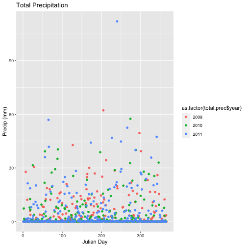
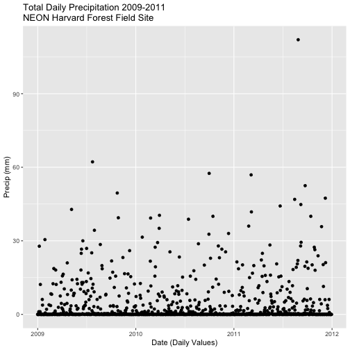
- Calculate total
precfor each Julian Day over the 3 years - name your data_frametotal.prec. - Create a plot of Daily Total Precipitation for 2009-2011.
- Add a title and x and y axis labels.
- If you use
qplotto create your plot, usecolour=as.factor(total.prec$year)to color the data points by year.
## `summarise()` has grouped output by 'year'. You can override using the `.groups` argument.
Mutate - Add data_frame Columns to dplyr Output
We can use the mutate() function of dplyr to add additional columns of
information to a data_frame. For instance, we added the year column
independently at the very beginning of the tutorial. However, we can add the
year using a dplyr pipe that also summarizes our data. To do this, we would
use the syntax:
mutate(year2 = year(datetime))
year2 is the name of the column that will be added to the output dplyr
data_frame.
harMet15.09.11 %>%
mutate(year2 = year(datetime)) %>%
group_by(year2, jd) %>%
dplyr::summarize(mean_airt = mean(airt, na.rm = TRUE))
## `summarise()` has grouped output by 'year2'. You can override using the `.groups` argument.
## # A tibble: 1,096 x 3
## # Groups: year2 [3]
## year2 jd mean_airt
## <dbl> <int> <dbl>
## 1 2009 1 -15.1
## 2 2009 2 -9.14
## 3 2009 3 -5.54
## 4 2009 4 -6.35
## 5 2009 5 -2.41
## 6 2009 6 -4.92
## 7 2009 7 -2.59
## 8 2009 8 -3.23
## 9 2009 9 -9.92
## 10 2009 10 -11.1
## # � with 1,086 more rows
Save dplyr Output as data_frame
We can save output from a dplyr pipe as a new R object to use for quick
plotting.
harTemp.daily.09.11<-harMet15.09.11 %>%
                    mutate(year2 = year(datetime)) %>%
                    group_by(year2, jd) %>%
                    dplyr::summarize(mean_airt = mean(airt, na.rm = TRUE))

## `summarise()` has grouped output by 'year2'. You can override using the `.groups` argument.

head(harTemp.daily.09.11)

## # A tibble: 6 x 3
## # Groups:   year2 [1]
##   year2    jd mean_airt
##   <dbl> <int>     <dbl>
## 1  2009     1    -15.1
## 2  2009     2     -9.14
## 3  2009     3     -5.54
## 4  2009     4     -6.35
## 5  2009     5     -2.41
## 6  2009     6     -4.92
Add Date-Time To dplyr Output
In the challenge above, we created a plot of daily precipitation data using
qplot. However, the x-axis ranged from 0-366 (Julian Days for the year). It
would have been easier to create a meaningful plot across all three years if we
had a continuous date variable in our data_frame representing the year and
date for each summary value.
We can add the the datetime column value to our data_frame by adding an
additional argument to the summarize() function. In this case, we will add the
first datetime value that R encounters when summarizing data by group as
follows:
datetime = first(datetime)
Our new summarize statement in our pipe will look like this:
summarize(mean_airt = mean(airt, na.rm = TRUE), datetime = first(datetime))
Let's try it!
# add in a datatime column
harTemp.daily.09.11 <- harMet15.09.11 %>%
mutate(year3 = year(datetime)) %>%
group_by(year3, jd) %>%
dplyr::summarize(mean_airt = mean(airt, na.rm = TRUE), datetime = first(datetime))
## `summarise()` has grouped output by 'year3'. You can override using the `.groups` argument.
# view str and head of data
str(harTemp.daily.09.11)
## tibble [1,096 Ă— 4] (S3: grouped_df/tbl_df/tbl/data.frame)
## $ year3 : num [1:1096] 2009 2009 2009 2009 2009 ...
## $ jd : int [1:1096] 1 2 3 4 5 6 7 8 9 10 ...
## $ mean_airt: num [1:1096] -15.13 -9.14 -5.54 -6.35 -2.41 ...
## $ datetime : POSIXct[1:1096], format: "2009-01-01 00:15:00" ...
## - attr(*, "groups")= tibble [3 Ă— 2] (S3: tbl_df/tbl/data.frame)
## ..$ year3: num [1:3] 2009 2010 2011
## ..$ .rows: list<int> [1:3]
## .. ..$ : int [1:366] 1 2 3 4 5 6 7 8 9 10 ...
## .. ..$ : int [1:365] 367 368 369 370 371 372 373 374 375 376 ...
## .. ..$ : int [1:365] 732 733 734 735 736 737 738 739 740 741 ...
## .. ..@ ptype: int(0)
## ..- attr(*, ".drop")= logi TRUE
head(harTemp.daily.09.11)
## # A tibble: 6 x 4
## # Groups: year3 [1]
## year3 jd mean_airt datetime
## <dbl> <int> <dbl> <dttm>
## 1 2009 1 -15.1 2009-01-01 00:15:00
## 2 2009 2 -9.14 2009-01-02 00:15:00
## 3 2009 3 -5.54 2009-01-03 00:15:00
## 4 2009 4 -6.35 2009-01-04 00:15:00
## 5 2009 5 -2.41 2009-01-05 00:15:00
## 6 2009 6 -4.92 2009-01-06 00:15:00
- Plot daily total precipitation from 2009-2011 as we did in the previous challenge. However this time, use the new syntax that you learned (mutate and summarize to add a datetime column to your output data_frame).
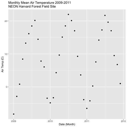
- Create a data_frame of the average monthly air temperature for 2009-2011.
Name the new data frame
harTemp.monthly.09.11. Plot your output.
## `summarise()` has grouped output by 'year'. You can override using the `.groups` argument.
## `summarise()` has grouped output by 'month'. You can override using the `.groups` argument.