Tutorial
Vector 03: When Vector Data Don't Line Up - Handling Spatial Projection & CRS in R
Last Updated: Apr 8, 2021
In this tutorial, we will create a base map of our study site using a United States
state and country boundary accessed from the
.
We will learn how to map vector data that are in different CRS and thus
don't line up on a map.
Learning Objectives
After completing this tutorial, you will be able to:
- Identify the
CRSof a spatial dataset. - Differentiate between with geographic vs. projected coordinate reference systems.
- Use the
proj4string format which is one format used used to store & reference theCRSof a spatial object.
Things You’ll Need To Complete This Tutorial
You will need the most current version of R and, preferably, RStudio loaded
on your computer to complete this tutorial.
Install R Packages
-
raster:
install.packages("raster") -
rgdal:
install.packages("rgdal") -
sp:
install.packages("sp") -
More on Packages in R � Adapted from Software Carpentry.
Data to Download
These vector data provide information on the site characterization and infrastructure at the National Ecological Observatory Network's Harvard Forest field site. The Harvard Forest shapefiles are from the archives. US Country and State Boundary layers are from the .
The LiDAR and imagery data used to create this raster teaching data subset were collected over the National Ecological Observatory Network's Harvard Forest and San Joaquin Experimental Range field sites and processed at NEON headquarters. The entire dataset can be accessed by request from the .
Set Working Directory: This lesson assumes that you have set your working directory to the location of the downloaded and unzipped data subsets.
An overview of setting the working directory in R can be found here.
R Script & Challenge Code: NEON data lessons often contain challenges that reinforce learned skills. If available, the code for challenge solutions is found in the downloadable R script of the entire lesson, available in the footer of each lesson page.
Working With Spatial Data From Different Sources
To support a project, we often need to gather spatial datasets for from
different sources and/or data that cover different spatial extents. Spatial
data from different sources and that cover different extents are often in
different Coordinate Reference Systems (CRS).
Some reasons for data being in different CRS include:
- The data are stored in a particular CRS convention used by the data provider; perhaps a federal agency or a state planning office.
- The data are stored in a particular CRS that is customized to a region. For instance, many states prefer to use a State Plane projection customized for that state.
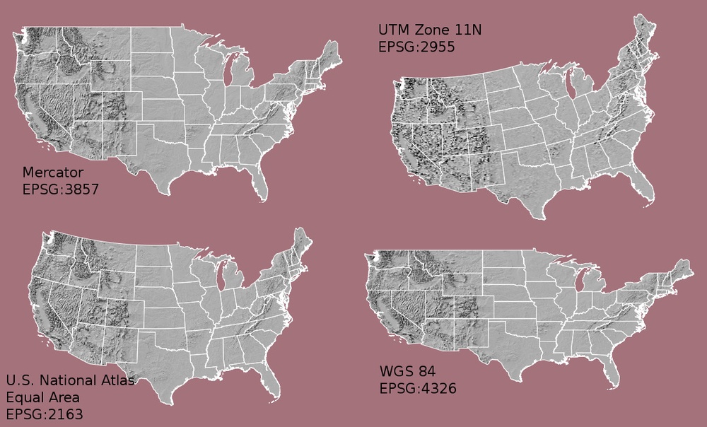
Check out this short video from highlighting how map projections can make continents seems proportionally larger or smaller than they actually are!
In this tutorial we will learn how to identify and manage spatial data
in different projections. We will learn how to reproject the data so that they
are in the same projection to support plotting / mapping. Note that these skills
are also required for any geoprocessing / spatial analysis, as data need to be in
the same CRS to ensure accurate results.
We will use the rgdal and raster libraries in this tutorial.
# load packages
library(rgdal)  # for vector work; sp package should always load with rgdal.
library (raster)   # for metadata/attributes- vectors or rasters

# set working directory to data folder
# setwd("pathToDirHere")
Import US Boundaries - Census Data
There are many good sources of boundary base layers that we can use to create a basemap. Some R packages even have these base layers built in to support quick and efficient mapping. In this tutorial, we will use boundary layers for the United States, provided by the
It is useful to have shapefiles to work with because we can add additional attributes to them if need be - for project specific mapping.
Read US Boundary File
We will use the readOGR() function to import the
/US-Boundary-Layers/US-State-Boundaries-Census-2014 layer into R. This layer
contains the boundaries of all continental states in the U.S.. Please note that
these data have been modified and reprojected from the original data downloaded
from the Census website to support the learning goals of this tutorial.
# Read the .csv file
State.Boundary.US <- readOGR("NEON-DS-Site-Layout-Files/US-Boundary-Layers",
          "US-State-Boundaries-Census-2014")

## OGR data source with driver: ESRI Shapefile
## Source: "/Users/olearyd/Git/data/NEON-DS-Site-Layout-Files/US-Boundary-Layers", layer: "US-State-Boundaries-Census-2014"
## with 58 features
## It has 10 fields
## Integer64 fields read as strings:  ALAND AWATER

## Warning in readOGR("NEON-DS-Site-Layout-Files/US-Boundary-Layers", "US-
## State-Boundaries-Census-2014"): Z-dimension discarded

# look at the data structure
class(State.Boundary.US)

## [1] "SpatialPolygonsDataFrame"
## attr(,"package")
## [1] "sp"
Note: the Z-dimension warning is normal. The readOGR() function doesn't import
z (vertical dimension or height) data by default. This is because not all
shapefiles contain z dimension data.
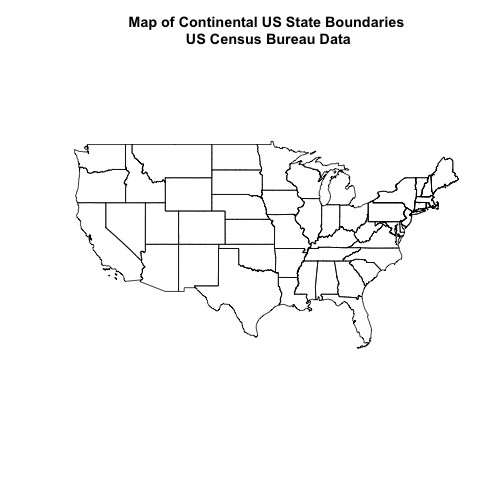
Now, let's plot the U.S. states data.
# view column names
plot(State.Boundary.US,
     main="Map of Continental US State Boundaries\n US Census Bureau Data")
U.S. Boundary Layer
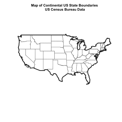
We can add a boundary layer of the United States to our map to make it look
nicer. We will import
NEON-DS-Site-Layout-Files/US-Boundary-Layers/US-Boundary-Dissolved-States.
If we specify a thicker line width using lwd=4 for the border layer, it will
make our map pop!
# Read the .csv file
Country.Boundary.US <- readOGR("NEON-DS-Site-Layout-Files/US-Boundary-Layers",
          "US-Boundary-Dissolved-States")

## OGR data source with driver: ESRI Shapefile
## Source: "/Users/olearyd/Git/data/NEON-DS-Site-Layout-Files/US-Boundary-Layers", layer: "US-Boundary-Dissolved-States"
## with 1 features
## It has 9 fields
## Integer64 fields read as strings:  ALAND AWATER

## Warning in readOGR("NEON-DS-Site-Layout-Files/US-Boundary-Layers", "US-
## Boundary-Dissolved-States"): Z-dimension discarded

# look at the data structure
class(Country.Boundary.US)

## [1] "SpatialPolygonsDataFrame"
## attr(,"package")
## [1] "sp"

# view column names
plot(State.Boundary.US,
     main="Map of Continental US State Boundaries\n US Census Bureau Data",
     border="gray40")

# view column names
plot(Country.Boundary.US,
     lwd=4,
     border="gray18",
     add=TRUE)
Next, let's add the location of a flux tower where our study area is. As we are adding these layers, take note of the class of each object.
# Import a point shapefile
point_HARV <- readOGR("NEON-DS-Site-Layout-Files/HARV/",
                      "HARVtower_UTM18N")

## OGR data source with driver: ESRI Shapefile
## Source: "/Users/olearyd/Git/data/NEON-DS-Site-Layout-Files/HARV", layer: "HARVtower_UTM18N"
## with 1 features
## It has 14 fields

class(point_HARV)

## [1] "SpatialPointsDataFrame"
## attr(,"package")
## [1] "sp"

# plot point - looks ok?
plot(point_HARV,
     pch = 19,
     col = "purple",
     main="Harvard Fisher Tower Location")
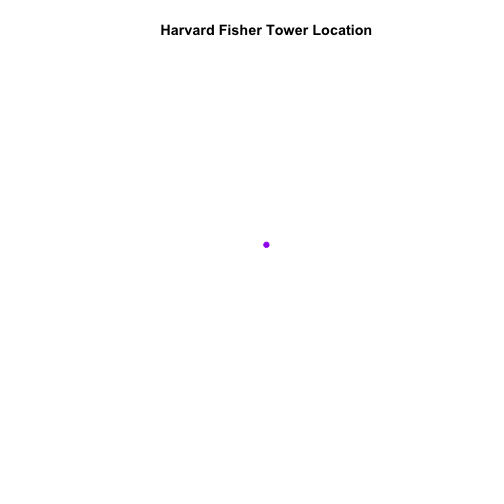
The plot above demonstrates that the tower point location data are readable and will plot! Let's next add it as a layer on top of the U.S. states and boundary layers in our basemap plot.
# plot state boundaries
plot(State.Boundary.US,
     main="Map of Continental US State Boundaries \n with Tower Location",
     border="gray40")

# add US border outline
plot(Country.Boundary.US,
     lwd=4,
     border="gray18",
     add=TRUE)

# add point tower location
plot(point_HARV,
     pch = 19,
     col = "purple",
     add=TRUE)
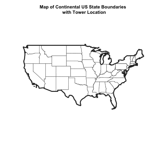
What do you notice about the resultant plot? Do you see the tower location in purple in the Massachusetts area? No! So what went wrong?
Let's check out the CRS (crs()) of both datasets to see if we can identify any
issues that might cause the point location to not plot properly on top of our
U.S. boundary layers.
# view CRS of our site data
crs(point_HARV)

## CRS arguments:
##  +proj=utm +zone=18 +datum=WGS84 +units=m +no_defs

# view crs of census data
crs(State.Boundary.US)

## CRS arguments: +proj=longlat +datum=WGS84 +no_defs

crs(Country.Boundary.US)

## CRS arguments: +proj=longlat +datum=WGS84 +no_defs
It looks like our data are in different CRS. We can tell this by looking at
the CRS strings in proj4 format.
Understanding CRS in Proj4 Format
The CRS for our data are given to us by R in proj4 format. Let's break
down the pieces of proj4 string. The string contains all of the individual
CRS elements that R or another GIS might need. Each element is specified
with a + sign, similar to how a .csv file is delimited or broken up by
a ,. After each + we see the CRS element being defined. For example
projection (proj=) and datum (datum=).
UTM Proj4 String
Our project string for point_HARV specifies the UTM projection as follows:
+proj=utm +zone=18 +datum=WGS84 +units=m +no_defs +ellps=WGS84 +towgs84=0,0,0
- proj=utm: the projection is UTM
- zone=18: the zone is 18
- datum=WGS84: the datum WGS84 (the datum refers to the 0,0 reference for the coordinate system used in the projection)
- units=m: the units for the coordinates are in METERS
- ellps=WGS84: the ellipsoid (how the earth's roundness is calculated) for the data is WGS84
Note that the zone is unique to the UTM projection. Not all CRS will have a
zone.
Geographic (lat / long) Proj4 String
Our project string for State.boundary.US and Country.boundary.US specifies
the lat/long projection as follows:
+proj=longlat +datum=WGS84 +no_defs +ellps=WGS84 +towgs84=0,0,0
- proj=longlat: the data are in a geographic (latitude and longitude) coordinate system
- datum=WGS84: the datum is WGS84
- ellps=WGS84: the ellipsoid is WGS84
Note that there are no specified units above. This is because this geographic coordinate reference system is in latitude and longitude which is most often recorded in Decimal Degrees.
CRS Units - View Object Extent
Next, let's view the extent or spatial coverage for the point_HARV spatial
object compared to the State.Boundary.US object.
# extent for HARV in UTM
extent(point_HARV)

## class      : Extent
## xmin       : 732183.2
## xmax       : 732183.2
## ymin       : 4713265
## ymax       : 4713265

# extent for object in geographic
extent(State.Boundary.US)

## class      : Extent
## xmin       : -124.7258
## xmax       : -66.94989
## ymin       : 24.49813
## ymax       : 49.38436
Note the difference in the units for each object. The extent for
State.Boundary.US is in latitude and longitude, which yields smaller numbers
representing decimal degree units; however, our tower location point
is in UTM, which is represented in meters.
Proj4 & CRS Resources
- To view a list of datum conversion factors, type
projInfo(type = "datum")into the R console.
Reproject Vector Data
Now we know our data are in different CRS. To address this, we have to modify
or reproject the data so they are all in the same CRS. We can use
spTransform() function to reproject our data. When we reproject the data, we
specify the CRS that we wish to transform our data to. This CRS contains
the datum, units and other information that R needs to reproject our data.
The spTransform() function requires two inputs:
- The name of the object that you wish to transform
- The CRS that you wish to transform that object too. In this case we can
use the
crs()of theState.Boundary.USobject as follows:crs(State.Boundary.US)
Next, let's reproject our point layer into the geographic latitude and
longitude WGS84 coordinate reference system (CRS).
# reproject data
point_HARV_WGS84 <- spTransform(point_HARV,
                                crs(State.Boundary.US))

# what is the CRS of the new object
crs(point_HARV_WGS84)

## CRS arguments: +proj=longlat +datum=WGS84 +no_defs

# does the extent look like decimal degrees?
extent(point_HARV_WGS84)

## class      : Extent
## xmin       : -72.17266
## xmax       : -72.17266
## ymin       : 42.5369
## ymax       : 42.5369
Once our data are reprojected, we can try to plot again.
# plot state boundaries
plot(State.Boundary.US,
     main="Map of Continental US State Boundaries\n With Fisher Tower Location",
     border="gray40")

# add US border outline
plot(Country.Boundary.US,
     lwd=4,
     border="gray18",
     add=TRUE)

# add point tower location
plot(point_HARV_WGS84,
     pch = 19,
     col = "purple",
     add=TRUE)
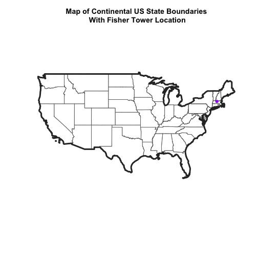
Reprojecting our data ensured that things line up on our map! It will also allow us to perform any required geoprocessing (spatial calculations / transformations) on our data.
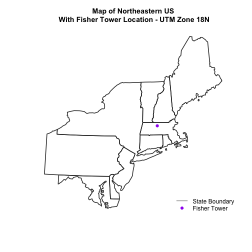
Create a map of the North Eastern United States as follows:
- Import and plot
Boundary-US-State-NEast.shp. Adjust line width as necessary. - Reproject the layer into UTM zone 18 north.
- Layer the Fisher Tower point location
point_HARVon top of the above plot. - Add a title to your plot.
- Add a legend to your plot that shows both the state boundary (line) and the Tower location point.