Series
Intro to Vector Data in R
The data tutorials in this series cover how to open, work with and plot vector-format spatial data (points, lines and polygons) in R. Additional topics include working with spatial metadata (extent and coordinate reference system), working with spatial attributes and plotting data by attribute.
Data used in this series cover NEON Harvard Forest Field Site and are in shapefile and .csv formats.
Learning Objectives
After completing the series you will:
-
Vector 00:
- Know the difference between point, line, and polygon vector elements.
- Understand the differences between opening point, line and polygon shapefiles in R.
-
Vector 01:
- Understand the components of a spatial object in R.
- Be able to query shapefile attributes.
- Be able to subset shapefiles using specific attribute values.
- Know how to plot a shapefile, colored by unique attribute values.
-
Vector 02:
- Be able to plot multiple shapefiles using base
plot(). - Be able to apply custom symbology to spatial objects in a plot in R.
- Be able to customize a baseplot legend in R.
- Be able to plot multiple shapefiles using base
-
Vector 03:
- Know how to identify the CRS of a spatial dataset.
- Be familiar with geographic vs. projected coordinate reference systems.
- Be familiar with the proj4 string format which is one format used used to store / reference the CRS of a spatial object.
-
Vector 04:
- Be able to import .csv files containing x,y coordinate locations into R.
- Know how to convert a .csv to a spatial object.
- Understand how to project coordinate locations provided in a Geographic Coordinate System (Latitude, Longitude) to a projected coordinate system (UTM).
- Be able to plot raster and vector data in the same plot to create a map.
-
Vector 05:
- Be able to crop a raster to the extent of a vector layer.
- Be able to extract values from raster that correspond to a vector file overlay.
Things You’ll Need To Complete This Series
Setup RStudio
To complete the tutorial series you will need an updated version of R and,
preferably, RStudio installed on your computer.
is a programming language that specializes in statistical computing. It is a
powerful tool for exploratory data analysis. To interact with R, we strongly
recommend
,
an interactive development environment (IDE).
Install R Packages
You can chose to install packages with each lesson or you can download all of the necessary R packages now.
-
raster:
install.packages("raster") -
rgdal:
install.packages("rgdal") -
sp:
install.packages("sp")
More on Packages in R � Adapted from Software Carpentry.
Working with Vector Data in R Tutorial Series: This is part of a larger collection of spatio-temporal data tutorials. It is also part of a Data Carpentry workshop: on using spatio-temporal in R. Other related series include Data Carpentry's , and NEON's Working with Tabular Time Series Data in R .
Vector 00: Open and Plot Shapefiles in R - Getting Started with Point, Line and Polygon Vector Data
Last Updated: Apr 8, 2021
In this tutorial, we will open and plot point, line and polygon vector data stored in shapefile format in R.
Learning Objectives
After completing this tutorial, you will be able to:
- Explain the difference between point, line, and polygon vector elements.
- Describe the differences between opening point, line and polygon shapefiles in R.
- Describe the components of a spatial object in R.
- Read a shapefile into R.
Things You’ll Need To Complete This Tutorial
You will need the most current version of R and, preferably, RStudio loaded
on your computer to complete this tutorial.
Install R Packages
-
raster:
install.packages("raster") -
rgdal:
install.packages("rgdal") -
sp:
install.packages("sp")
More on Packages in R � Adapted from Software Carpentry.
Download Data
These vector data provide information on the site characterization and infrastructure at the National Ecological Observatory Network's Harvard Forest field site. The Harvard Forest shapefiles are from the archives. US Country and State Boundary layers are from the .
Set Working Directory: This lesson assumes that you have set your working directory to the location of the downloaded and unzipped data subsets.
An overview of setting the working directory in R can be found here.
R Script & Challenge Code: NEON data lessons often contain challenges that reinforce learned skills. If available, the code for challenge solutions is found in the downloadable R script of the entire lesson, available in the footer of each lesson page.
AGŐćČË°ŮĽŇŔֹٷ˝ÍřŐľ Vector Data
Vector data are composed of discrete geometric locations (x,y values) known as vertices that define the "shape" of the spatial object. The organization of the vertices, determines the type of vector that we are working with: point, line or polygon.
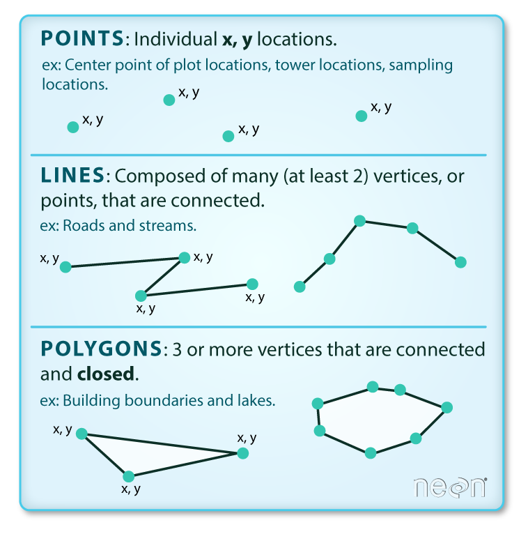
- Points: Each individual point is defined by a single x, y coordinate. There can be many points in a vector point file. Examples of point data include: sampling locations, the location of individual trees or the location of plots.
-
Lines: Lines are composed of many (at least 2) vertices, or points, that
are connected. For instance, a road or a stream may be represented by a line. This
line is composed of a series of segments, each "bend" in the road or stream
represents a vertex that has defined
x, ylocation. - Polygons: A polygon consists of 3 or more vertices that are connected and "closed". Thus the outlines of plot boundaries, lakes, oceans, and states or countries are often represented by polygons. Occasionally, a polygon can have a hole in the middle of it (like a doughnut), this is something to be aware of but not an issue we will deal with in this tutorial.
Shapefiles: Points, Lines, and Polygons
Geospatial data in vector format are often stored in a shapefile format.
Because the structure of points, lines, and polygons are different, each
individual shapefile can only contain one vector type (all points, all lines
or all polygons). You will not find a mixture of point, line and polygon
objects in a single shapefile.
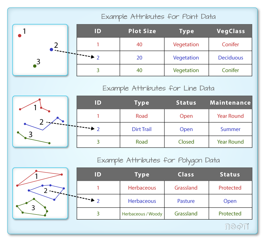
Objects stored in a shapefile often have a set of associated attributes that
describe the data. For example, a line shapefile that contains the locations of
streams, might contain the associated stream name, stream "order" and other
information about each stream line object.
- More about shapefiles can found on .
Import Shapefiles
We will use the rgdal package to work with vector data in R. Notice that the
sp package automatically loads when rgdal is loaded. We will also load the
raster package so we can explore raster and vector spatial metadata using similar commands.
# load required libraries
# for vector work; sp package will load with rgdal.
library(rgdal)
# for metadata/attributes- vectors or rasters
library(raster)

# set working directory to the directory location on your computer where
# you downloaded and unzipped the data files for the tutorial
# setwd("pathToDirHere")
The shapefiles that we will import are:
- A polygon shapefile representing our field site boundary,
- A line shapefile representing roads, and
- A point shapefile representing the location of the Fisher
flux tower located at the NEON Harvard Forest field site.
The first shapefile that we will open contains the boundary of our study area
(or our Area Of Interest or AOI, hence the name aoiBoundary). To import
shapefiles we use the R function readOGR().
readOGR() requires two components:
- The directory where our shapefile lives:
NEON-DS-Site-Layout-Files/HARV - The name of the shapefile (without the extension):
HarClip_UTMZ18
Let's import our AOI.
# Import a polygon shapefile: readOGR("path","fileName")
# no extension needed as readOGR only imports shapefiles
aoiBoundary_HARV <- readOGR(dsn=path.expand("NEON-DS-Site-Layout-Files/HARV"),
                            layer="HarClip_UTMZ18")

## OGR data source with driver: ESRI Shapefile
## Source: "/Users/olearyd/Git/data/NEON-DS-Site-Layout-Files/HARV", layer: "HarClip_UTMZ18"
## with 1 features
## It has 1 fields
## Integer64 fields read as strings:  id
Shapefile Metadata & Attributes
When we import the HarClip_UTMZ18 shapefile layer into R (as our
aoiBoundary_HARV object), the readOGR() function automatically stores
information about the data. We are particularly interested in the geospatial
metadata, describing the format, CRS, extent, and other components of
the vector data, and the attributes which describe properties associated
with each individual vector object.
Spatial Metadata
Key metadata for all shapefiles include:
- Object Type: the class of the imported object.
- Coordinate Reference System (CRS): the projection of the data.
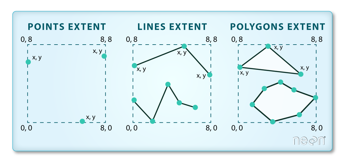
- Extent: the spatial extent (geographic area that the shapefile covers) of the shapefile. Note that the spatial extent for a shapefile represents the extent for ALL spatial objects in the shapefile.
We can view shapefile metadata using the class, crs and extent methods:
# view just the class for the shapefile
class(aoiBoundary_HARV)

## [1] "SpatialPolygonsDataFrame"
## attr(,"package")
## [1] "sp"

# view just the crs for the shapefile
crs(aoiBoundary_HARV)

## CRS arguments:
##  +proj=utm +zone=18 +datum=WGS84 +units=m +no_defs

# view just the extent for the shapefile
extent(aoiBoundary_HARV)

## class      : Extent
## xmin       : 732128
## xmax       : 732251.1
## ymin       : 4713209
## ymax       : 4713359

# view all metadata at same time
aoiBoundary_HARV

## class       : SpatialPolygonsDataFrame
## features    : 1
## extent      : 732128, 732251.1, 4713209, 4713359  (xmin, xmax, ymin, ymax)
## crs         : +proj=utm +zone=18 +datum=WGS84 +units=m +no_defs
## variables   : 1
## names       : id
## value       :  1
Our aoiBoundary_HARV object is a polygon of class SpatialPolygonsDataFrame,
in the CRS UTM zone 18N. The CRS is critical to interpreting the object
extent values as it specifies units.
Spatial Data Attributes
Each object in a shapefile has one or more attributes associated with it. Shapefile attributes are similar to fields or columns in a spreadsheet. Each row in the spreadsheet has a set of columns associated with it that describe the row element. In the case of a shapefile, each row represents a spatial object - for example, a road, represented as a line in a line shapefile, will have one "row" of attributes associated with it. These attributes can include different types of information that describe objects stored within a shapefile. Thus, our road, may have a name, length, number of lanes, speed limit, type of road and other attributes stored with it.
We view the attributes of a SpatialPolygonsDataFrame using objectName@data
(e.g., aoiBoundary_HARV@data).
# alternate way to view attributes
aoiBoundary_HARV@data

##   id
## 0  1
In this case, our polygon object only has one attribute: id.
Metadata & Attribute Summary
We can view a metadata & attribute summary of each shapefile by entering
the name of the R object in the console. Note that the metadata output
includes the class, the number of features, the extent, and the
coordinate reference system (crs) of the R object. The last two lines of
summary show a preview of the R object attributes.
# view a summary of metadata & attributes associated with the spatial object
summary(aoiBoundary_HARV)

## Object of class SpatialPolygonsDataFrame
## Coordinates:
##       min       max
## x  732128  732251.1
## y 4713209 4713359.2
## Is projected: TRUE
## proj4string :
## [+proj=utm +zone=18 +datum=WGS84 +units=m +no_defs]
## Data attributes:
##       id
##  Length:1
##  Class :character
##  Mode  :character
Plot a Shapefile
Next, let's visualize the data in our R spatialpolygonsdataframe object using
plot().
# create a plot of the shapefile
# 'lwd' sets the line width
# 'col' sets internal color
# 'border' sets line color
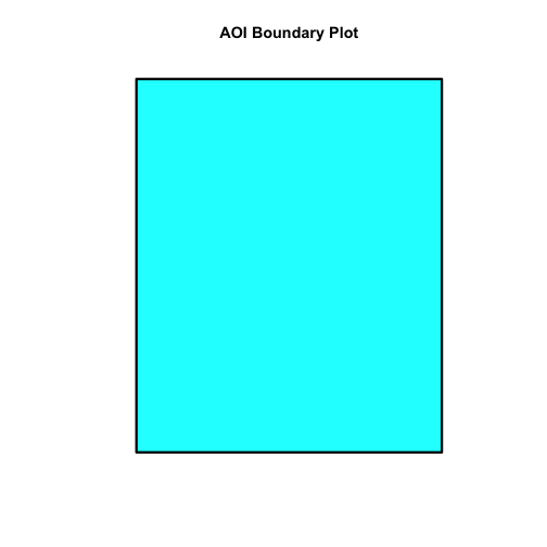
plot(aoiBoundary_HARV, col="cyan1", border="black", lwd=3,
main="AOI Boundary Plot")
Answer the following questions:
- What type of R spatial object is created when you import each layer?
- What is the
CRSandextentfor each object? - Do the files contain, points, lines or polygons?
- How many spatial objects are in each file?
Plot Multiple Shapefiles
The plot() function can be used for basic plotting of spatial objects.
We use the add = TRUE argument to overlay shapefiles on top of each other, as
we would when creating a map in a typical GIS application like QGIS.
We can use main="" to give our plot a title. If we want the title to span two
lines, we use \n where the line should break.
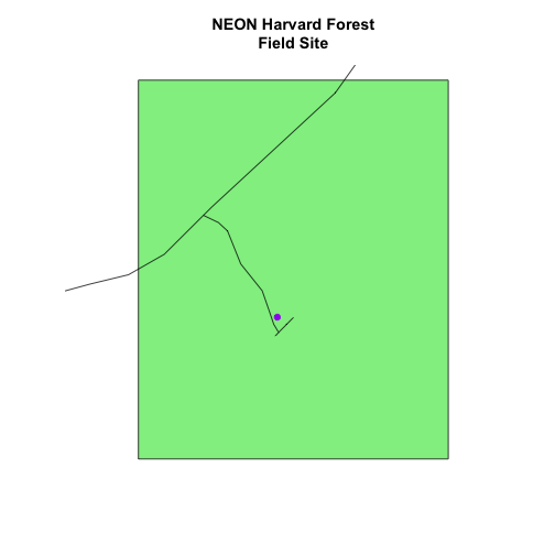
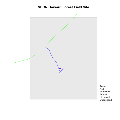
# Plot multiple shapefiles
plot(aoiBoundary_HARV, col = "lightgreen",
     main="NEON Harvard Forest\nField Site")
plot(lines_HARV, add = TRUE)

# use the pch element to adjust the symbology of the points
plot(point_HARV, add  = TRUE, pch = 19, col = "purple")
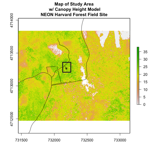
You can plot vector data layered on top of raster data using the add=TRUE
plot attribute. Create a plot that uses the NEON AOP Canopy Height Model NEON_RemoteSensing/HARV/CHM/HARV_chmCrop.tif as a base layer. On top of the
CHM, please add:
- The study site AOI.
- Roads.
- The tower location.
Be sure to give your plot a meaningful title.
For assistance consider using the Shapefile Metadata & Attributes in R and the Plot Raster Data in R tutorials.
Additional Resources: Plot Parameter Options
For more on parameter options in the base R plot() function, check out these
resources:
Get Lesson Code
Vector 01: Explore Shapefile Attributes & Plot Shapefile Objects by Attribute Value in R
Last Updated: Apr 8, 2021
This tutorial explains what shapefile attributes are and how to work with shapefile attributes in R. It also covers how to identify and query shapefile attributes, as well as subset shapefiles by specific attribute values. Finally, we will review how to plot a shapefile according to a set of attribute values.
Learning Objectives
After completing this tutorial, you will be able to:
- Query shapefile attributes.
- Subset shapefiles using specific attribute values.
- Plot a shapefile, colored by unique attribute values.
Things You’ll Need To Complete This Tutorial
You will need the most current version of R and, preferably, RStudio loaded
on your computer to complete this tutorial.
Install R Packages
-
raster:
install.packages("raster") -
rgdal:
install.packages("rgdal") -
sp:
install.packages("sp")
More on Packages in R � Adapted from Software Carpentry.
Download Data
These vector data provide information on the site characterization and infrastructure at the National Ecological Observatory Network's Harvard Forest field site. The Harvard Forest shapefiles are from the archives. US Country and State Boundary layers are from the .
Set Working Directory: This lesson assumes that you have set your working directory to the location of the downloaded and unzipped data subsets.
An overview of setting the working directory in R can be found here.
R Script & Challenge Code: NEON data lessons often contain challenges that reinforce learned skills. If available, the code for challenge solutions is found in the downloadable R script of the entire lesson, available in the footer of each lesson page.
Shapefile Metadata & Attributes
When we import a shapefile into R, the readOGR() function automatically
stores metadata and attributes associated with the file.
Load the Data
To work with vector data in R, we can use the rgdal library. The raster
package also allows us to explore metadata using similar commands for both
raster and vector files.
We will import three shapefiles. The first is our AOI or area of
interest boundary polygon that we worked with in
Open and Plot Shapefiles in R.
The second is a shapefile containing the location of roads and trails within the
field site. The third is a file containing the Fisher tower location.
If you completed the Open and Plot Shapefiles in R. tutorial, you can skip this code.
# load packages
# rgdal: for vector work; sp package should always load with rgdal.
library(rgdal)
# raster: for metadata/attributes- vectors or rasters
library (raster)

# set working directory to data folder
# setwd("pathToDirHere")

# Import a polygon shapefile
aoiBoundary_HARV <- readOGR("NEON-DS-Site-Layout-Files/HARV",
                            "HarClip_UTMZ18", stringsAsFactors = T)

## OGR data source with driver: ESRI Shapefile
## Source: "/Users/olearyd/Git/data/NEON-DS-Site-Layout-Files/HARV", layer: "HarClip_UTMZ18"
## with 1 features
## It has 1 fields
## Integer64 fields read as strings:  id

# Import a line shapefile
lines_HARV <- readOGR( "NEON-DS-Site-Layout-Files/HARV", "HARV_roads", stringsAsFactors = T)

## OGR data source with driver: ESRI Shapefile
## Source: "/Users/olearyd/Git/data/NEON-DS-Site-Layout-Files/HARV", layer: "HARV_roads"
## with 13 features
## It has 15 fields

# Import a point shapefile
point_HARV <- readOGR("NEON-DS-Site-Layout-Files/HARV",
                      "HARVtower_UTM18N", stringsAsFactors = T)

## OGR data source with driver: ESRI Shapefile
## Source: "/Users/olearyd/Git/data/NEON-DS-Site-Layout-Files/HARV", layer: "HARVtower_UTM18N"
## with 1 features
## It has 14 fields
Query Shapefile Metadata
Remember, as covered in Open and Plot Shapefiles in R., we can view metadata associated with an R object using:
-
class()- Describes the type of vector data stored in the object. -
length()- How many features are in this spatial object? - object
extent()- The spatial extent (geographic area covered by) features in the object. - coordinate reference system (
crs()) - The spatial projection that the data are in.
Let's explore the metadata for our point_HARV object.
# view class
class(x = point_HARV)

## [1] "SpatialPointsDataFrame"
## attr(,"package")
## [1] "sp"

# x= isn't actually needed; it just specifies which object
# view features count
length(point_HARV)

## [1] 1

# view crs - note - this only works with the raster package loaded
crs(point_HARV)

## CRS arguments:
##  +proj=utm +zone=18 +datum=WGS84 +units=m +no_defs

# view extent- note - this only works with the raster package loaded
extent(point_HARV)

## class      : Extent
## xmin       : 732183.2
## xmax       : 732183.2
## ymin       : 4713265
## ymax       : 4713265

# view metadata summary
point_HARV

## class       : SpatialPointsDataFrame
## features    : 1
## extent      : 732183.2, 732183.2, 4713265, 4713265  (xmin, xmax, ymin, ymax)
## crs         : +proj=utm +zone=18 +datum=WGS84 +units=m +no_defs
## variables   : 14
## names       : Un_ID, Domain, DomainName,       SiteName, Type,       Sub_Type,     Lat,      Long, Zone,       Easting,       Northing,                Ownership,    County, annotation
## value       :     A,      1,  Northeast, Harvard Forest, Core, Advanced Tower, 42.5369, -72.17266,   18, 732183.193774, 4713265.041137, Harvard University, LTER, Worcester,         C1
AGŐćČË°ŮĽŇŔֹٷ˝ÍřŐľ Shapefile Attributes
Shapefiles often contain an associated database or spreadsheet of values called attributes that describe the vector features in the shapefile. You can think of this like a spreadsheet with rows and columns. Each column in the spreadsheet is an individual attribute that describes an object. Shapefile attributes include measurements that correspond to the geometry of the shapefile features.
For example, the HARV_Roads shapefile (lines_HARV object) contains an
attribute called TYPE. Each line in the shapefile has an associated TYPE
which describes the type of road (woods road, footpath, boardwalk, or
stone wall).
We can look at all of the associated data attributes by printing the contents of
the data slot with objectName@data. We can use the base R length
function to count the number of attributes associated with a spatial object too.
# just view the attributes & first 6 attribute values of the data
head(lines_HARV@data)

##   OBJECTID_1 OBJECTID       TYPE             NOTES MISCNOTES RULEID
## 0         14       48 woods road Locust Opening Rd      <NA>      5
## 1         40       91   footpath              <NA>      <NA>      6
## 2         41      106   footpath              <NA>      <NA>      6
## 3        211      279 stone wall              <NA>      <NA>      1
## 4        212      280 stone wall              <NA>      <NA>      1
## 5        213      281 stone wall              <NA>      <NA>      1
##            MAPLABEL SHAPE_LENG             LABEL BIKEHORSE RESVEHICLE
## 0 Locust Opening Rd 1297.35706 Locust Opening Rd         Y         R1
## 1              <NA>  146.29984              <NA>         Y         R1
## 2              <NA>  676.71804              <NA>         Y         R2
## 3              <NA>  231.78957              <NA>      <NA>       <NA>
## 4              <NA>   45.50864              <NA>      <NA>       <NA>
## 5              <NA>  198.39043              <NA>      <NA>       <NA>
##   RECMAP Shape_Le_1                            ResVehic_1
## 0      Y 1297.10617    R1 - All Research Vehicles Allowed
## 1      Y  146.29983    R1 - All Research Vehicles Allowed
## 2      Y  676.71807 R2 - 4WD/High Clearance Vehicles Only
## 3   <NA>  231.78962                                  <NA>
## 4   <NA>   45.50859                                  <NA>
## 5   <NA>  198.39041                                  <NA>
##                    BicyclesHo
## 0 Bicycles and Horses Allowed
## 1 Bicycles and Horses Allowed
## 2 Bicycles and Horses Allowed
## 3                        <NA>
## 4                        <NA>
## 5                        <NA>

# how many attributes are in our vector data object?
length(lines_HARV@data)

## [1] 15
We can view the individual name of each attribute using the
names(lines_HARV@data) method in R. We could also view just the first 6 rows
of attribute values using head(lines_HARV@data).
Let's give it a try.
# view just the attribute names for the lines_HARV spatial object
names(lines_HARV@data)

##  [1] "OBJECTID_1" "OBJECTID"   "TYPE"       "NOTES"      "MISCNOTES"
##  [6] "RULEID"     "MAPLABEL"   "SHAPE_LENG" "LABEL"      "BIKEHORSE"
## [11] "RESVEHICLE" "RECMAP"     "Shape_Le_1" "ResVehic_1" "BicyclesHo"
-
How many attributes do each have?
-
Who owns the site in the
point_HARVdata object? -
Which of the following is NOT an attribute of the
pointdata object?A) Latitude B) County C) Country
Explore Values within One Attribute
We can explore individual values stored within a particular attribute.
Again, comparing attributes to a spreadsheet or a data.frame is similar
to exploring values in a column. We can do this using the $ and the name of
the attribute: objectName$attributeName.
# view all attributes in the lines shapefile within the TYPE field
lines_HARV$TYPE

##  [1] woods road footpath   footpath   stone wall stone wall stone wall
##  [7] stone wall stone wall stone wall boardwalk  woods road woods road
## [13] woods road
## Levels: boardwalk footpath stone wall woods road

# view unique values within the "TYPE" attributes
levels(lines_HARV@data$TYPE)

## [1] "boardwalk"  "footpath"   "stone wall" "woods road"
Notice that two of our TYPE attribute values consist of two separate words: stone wall and woods road. There are really four unique TYPE values, not six TYPE values.
Subset Shapefiles
We can use the objectName$attributeName syntax to select a subset of features
from a spatial object in R.
# select features that are of TYPE "footpath"
# could put this code into other function to only have that function work on
# "footpath" lines
lines_HARV[lines_HARV$TYPE == "footpath",]

## class       : SpatialLinesDataFrame
## features    : 2
## extent      : 731954.5, 732232.3, 4713131, 4713726  (xmin, xmax, ymin, ymax)
## crs         : +proj=utm +zone=18 +datum=WGS84 +units=m +no_defs
## variables   : 15
## names       : OBJECTID_1, OBJECTID,     TYPE, NOTES, MISCNOTES, RULEID, MAPLABEL,    SHAPE_LENG, LABEL, BIKEHORSE, RESVEHICLE, RECMAP,    Shape_Le_1,                            ResVehic_1,                  BicyclesHo
## min values  :         40,       91, footpath,    NA,        NA,      6,       NA, 146.299844868,    NA,         Y,         R1,      Y, 146.299831389,    R1 - All Research Vehicles Allowed, Bicycles and Horses Allowed
## max values  :         41,      106, footpath,    NA,        NA,      6,       NA,  676.71804248,    NA,         Y,         R2,      Y, 676.718065323, R2 - 4WD/High Clearance Vehicles Only, Bicycles and Horses Allowed

# save an object with only footpath lines
footpath_HARV <- lines_HARV[lines_HARV$TYPE == "footpath",]
footpath_HARV

## class       : SpatialLinesDataFrame
## features    : 2
## extent      : 731954.5, 732232.3, 4713131, 4713726  (xmin, xmax, ymin, ymax)
## crs         : +proj=utm +zone=18 +datum=WGS84 +units=m +no_defs
## variables   : 15
## names       : OBJECTID_1, OBJECTID,     TYPE, NOTES, MISCNOTES, RULEID, MAPLABEL,    SHAPE_LENG, LABEL, BIKEHORSE, RESVEHICLE, RECMAP,    Shape_Le_1,                            ResVehic_1,                  BicyclesHo
## min values  :         40,       91, footpath,    NA,        NA,      6,       NA, 146.299844868,    NA,         Y,         R1,      Y, 146.299831389,    R1 - All Research Vehicles Allowed, Bicycles and Horses Allowed
## max values  :         41,      106, footpath,    NA,        NA,      6,       NA,  676.71804248,    NA,         Y,         R2,      Y, 676.718065323, R2 - 4WD/High Clearance Vehicles Only, Bicycles and Horses Allowed

# how many features are in our new object
length(footpath_HARV)

## [1] 2
Our subsetting operation reduces the features count from 13 to 2. This means
that only two feature lines in our spatial object have the attribute
"TYPE=footpath".
We can plot our subsetted shapefiles.
# plot just footpaths
plot(footpath_HARV,
     lwd=6,
     main="NEON Harvard Forest Field Site\n Footpaths")
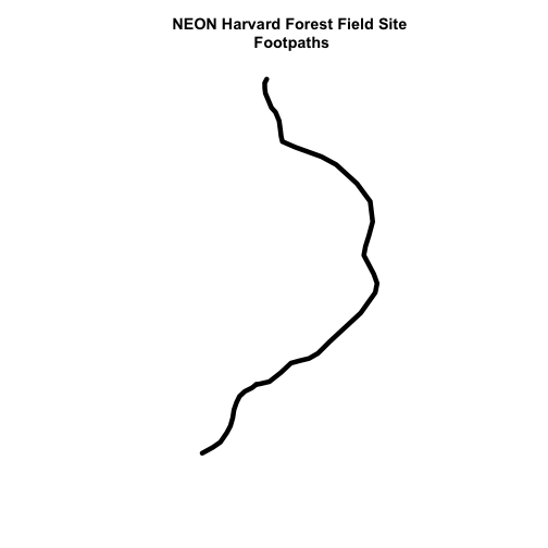
Interesting! Above, it appeared as if we had 2 features in our footpaths subset. Why does the plot look like there is only one feature?
Let's adjust the colors used in our plot. If we have 2 features in our vector
object, we can plot each using a unique color by assigning unique colors (col=)
to our features. We use the syntax
col="c("colorOne","colorTwo")
to do this.
# plot just footpaths
plot(footpath_HARV,
     col=c("green","blue"), # set color for each feature
     lwd=6,
     main="NEON Harvard Forest Field Site\n Footpaths \n Feature one = blue, Feature two= green")
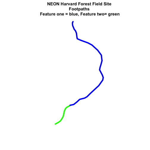
Now, we see that there are in fact two features in our plot!
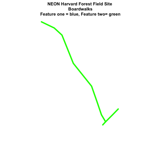
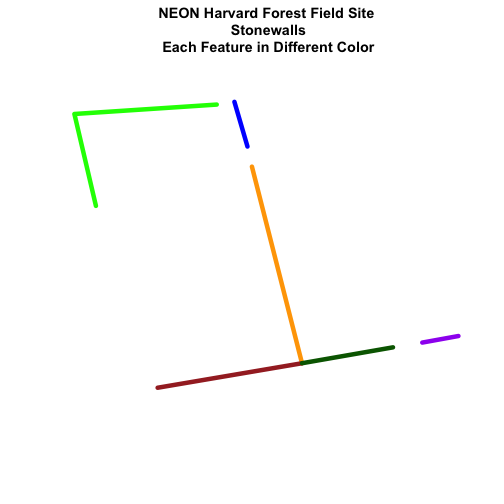
-
boardwalkfrom the lines layer and plot it. -
stone wallfeatures from the lines layer and plot it.
For each plot, color each feature using a unique color.
Plot Lines by Attribute Value
To plot vector data with the color determined by a set of attribute values, the
attribute values must be class = factor. A factor is similar to a category.
- you can group vector objects by a particular category value - for example you
can group all lines of
TYPE=footpath. However, in R, a factor can also have a determined order.
By default, R will import spatial object attributes as factors.
# view the original class of the TYPE column
class(lines_HARV$TYPE)

## [1] "factor"

# view levels or categories - note that there are no categories yet in our data!
# the attributes are just read as a list of character elements.
levels(lines_HARV$TYPE)

## [1] "boardwalk"  "footpath"   "stone wall" "woods road"

# Convert the TYPE attribute into a factor
# Only do this IF the data do not import as a factor!
# lines_HARV$TYPE <- as.factor(lines_HARV$TYPE)
# class(lines_HARV$TYPE)
# levels(lines_HARV$TYPE)

# how many features are in each category or level?
summary(lines_HARV$TYPE)

##  boardwalk   footpath stone wall woods road
##          1          2          6          4
When we use plot(), we can specify the colors to use for each attribute using
the col= element. To ensure that R renders each feature by it's associated
factor / attribute value, we need to create a vector or colors - one for each
feature, according to it's associated attribute value / factor value.
To create this vector we can use the following syntax:
c("colorOne", "colorTwo","colorThree")[object$factor]
Note in the above example we have:
- a vector of colors - one for each factor value (unique attribute value)
- the attribute itself (
[object$factor]) of classfactor
Let's give this a try.
# Check the class of the attribute - is it a factor?
class(lines_HARV$TYPE)
## [1] "factor"
# how many "levels" or unique values does the factor have?
# view factor values
levels(lines_HARV$TYPE)
## [1] "boardwalk" "footpath" "stone wall" "woods road"
# count the number of unique values or levels
length(levels(lines_HARV$TYPE))
## [1] 4
# create a color palette of 4 colors - one for each factor level
roadPalette <- c("blue","green","grey","purple")
roadPalette
## [1] "blue" "green" "grey" "purple"
# create a vector of colors - one for each feature in our vector object
# according to its attribute value
roadColors <- c("blue","green","grey","purple")[lines_HARV$TYPE]
roadColors
## [1] "purple" "green" "green" "grey" "grey" "grey" "grey"
## [8] "grey" "grey" "blue" "purple" "purple" "purple"
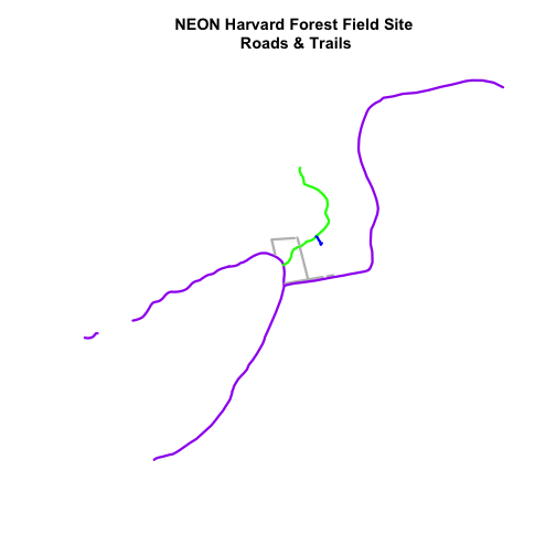
# plot the lines data, apply a diff color to each factor level)
plot(lines_HARV,
col=roadColors,
lwd=3,
main="NEON Harvard Forest Field Site\n Roads & Trails")
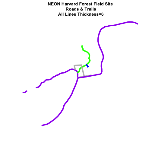
Adjust Line Width
We can also adjust the width of our plot lines using lwd. We can set all lines
to be thicker or thinner using lwd=.
# make all lines thicker
plot(lines_HARV,
     col=roadColors,
     main="NEON Harvard Forest Field Site\n Roads & Trails\n All Lines Thickness=6",
     lwd=6)
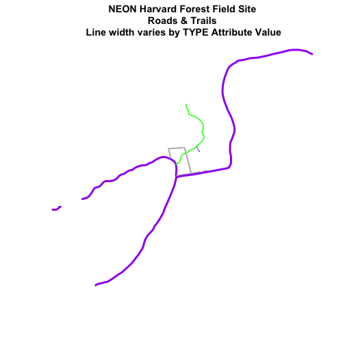
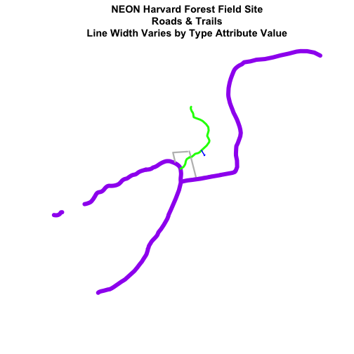
Adjust Line Width by Attribute
If we want a unique line width for each factor level or attribute category in our spatial object, we can use the same syntax that we used for colors, above:
lwd=c("widthOne", "widthTwo","widthThree")[object$factor]
Note that this requires the attribute to be of class factor. Let's give it a
try.
class(lines_HARV$TYPE)

## [1] "factor"

levels(lines_HARV$TYPE)

## [1] "boardwalk"  "footpath"   "stone wall" "woods road"

# create vector of line widths
lineWidths <- (c(1,2,3,4))[lines_HARV$TYPE]
# adjust line width by level
# in this case, boardwalk (the first level) is the widest.
plot(lines_HARV,
     col=roadColors,
     main="NEON Harvard Forest Field Site\n Roads & Trails \n Line width varies by TYPE Attribute Value",
     lwd=lineWidths)
Create a plot of roads using the following line thicknesses:
- woods road lwd=8
- Boardwalks lwd = 2
- footpath lwd=4
- stone wall lwd=3
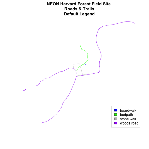
Add Plot Legend
We can add a legend to our plot too. When we add a legend, we use the following elements to specify labels and colors:
-
bottomright: We specify the location of our legend by using a default keyword. We could also usetop,topright, etc. -
levels(objectName$attributeName): Label the legend elements using the categories oflevelsin an attribute (e.g., levels(lines_HARV$TYPE) means use the levels boardwalk, footpath, etc). -
fill=: apply unique colors to the boxes in our legend.palette()is the default set of colors that R applies to all plots.
Let's add a legend to our plot.
plot(lines_HARV,
     col=roadColors,
     main="NEON Harvard Forest Field Site\n Roads & Trails\n Default Legend")

# we can use the color object that we created above to color the legend objects
roadPalette

## [1] "blue"   "green"  "grey"   "purple"

# add a legend to our map
legend("bottomright",   # location of legend
      legend=levels(lines_HARV$TYPE), # categories or elements to render in
			 # the legend
      fill=roadPalette) # color palette to use to fill objects in legend.
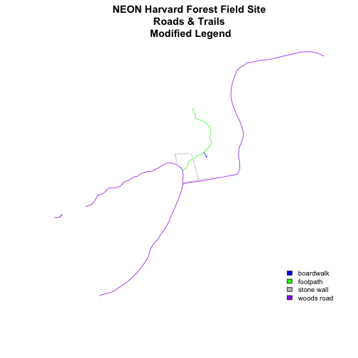
We can tweak the appearance of our legend too.
-
bty=n: turn off the legend BORDER -
cex: change the font size
Let's try it out.
plot(lines_HARV,
     col=roadColors,
     main="NEON Harvard Forest Field Site\n Roads & Trails \n Modified Legend")
# add a legend to our map
legend("bottomright",
       legend=levels(lines_HARV$TYPE),
       fill=roadPalette,
       bty="n", # turn off the legend border
       cex=.8) # decrease the font / legend size
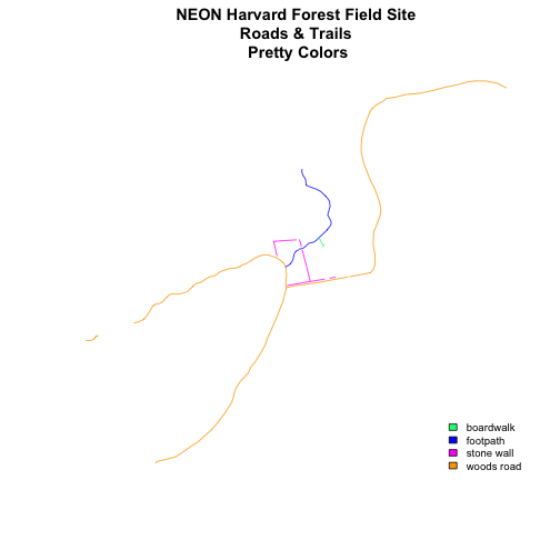
We can modify the colors used to plot our lines by creating a new color vector directly in the plot code rather than creating a separate object.
col=(newColors)[lines_HARV$TYPE]
Let's try it!
# manually set the colors for the plot!
newColors <- c("springgreen", "blue", "magenta", "orange")
newColors

## [1] "springgreen" "blue"        "magenta"     "orange"

# plot using new colors
plot(lines_HARV,
     col=(newColors)[lines_HARV$TYPE],
     main="NEON Harvard Forest Field Site\n Roads & Trails \n Pretty Colors")

# add a legend to our map
legend("bottomright",
       levels(lines_HARV$TYPE),
       fill=newColors,
       bty="n", cex=.8)
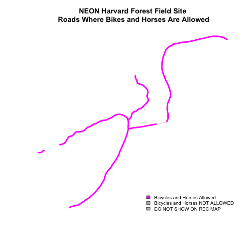
Be sure to add a title and legend to your map! You might consider a color palette that has all bike/horse-friendly roads displayed in a bright color. All other lines can be grey.
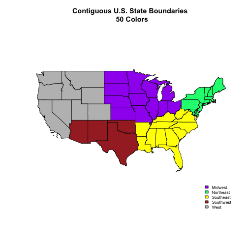
-
Create a map of the State boundaries in the United States using the data located in your downloaded data folder:
NEON-DS-Site-Layout-Files/US-Boundary-Layers\US-State-Boundaries-Census-2014. Apply a fill color to each state using itsregionvalue. Add a legend. -
Using the
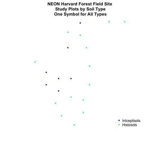
NEON-DS-Site-Layout-Files/HARV/PlotLocations_HARV.shpshapefile, create a map of study plot locations, with each point colored by the soil type (soilTypeOr). Question: How many different soil types are there at this particular field site? -
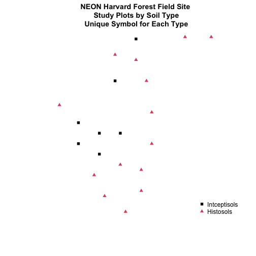
BONUS -- modify the field site plot above. Plot each point, using a different symbol. HINT: you can assign the symbol using
pch=value. You can create a vector object of symbols by factor level using the syntax syntax that we used above to create a vector of lines widths and colors:pch=c(15,17)[lines_HARV$soilTypeOr]. Type?pchto learn more about pch or use google to find a list of pch symbols that you can use in R.
Get Lesson Code
Vector 02: Plot Multiple Shapefiles and Create Custom Legends in Base Plot in R
Last Updated: Apr 8, 2021
This tutorial builds upon the previous tutorial, to work with shapefile attributes in R and explores how to plot multiple shapefiles using base R graphics. It then covers how to create a custom legend with colors and symbols that match your plot.
Learning Objectives
After completing this tutorial, you will be able to:
- Plot multiple shapefiles using base R graphics.
- Apply custom symbology to spatial objects in a plot in R.
- Customize a baseplot legend in R.
Things You’ll Need To Complete This Tutorial
You will need the most current version of R and preferably RStudio loaded
on your computer to complete this tutorial.
Install R Packages
-
raster:
install.packages("raster") -
rgdal:
install.packages("rgdal") -
sp:
install.packages("sp")
More on Packages in R � Adapted from Software Carpentry.
Download Data
These vector data provide information on the site characterization and infrastructure at the National Ecological Observatory Network's Harvard Forest field site. The Harvard Forest shapefiles are from the archives. US Country and State Boundary layers are from the .
Set Working Directory: This lesson assumes that you have set your working directory to the location of the downloaded and unzipped data subsets.
An overview of setting the working directory in R can be found here.
R Script & Challenge Code: NEON data lessons often contain challenges that reinforce learned skills. If available, the code for challenge solutions is found in the downloadable R script of the entire lesson, available in the footer of each lesson page.
Load the Data
To work with vector data in R, we can use the rgdal library. The raster
package also allows us to explore metadata using similar commands for both
raster and vector files.
We will import three shapefiles. The first is our AOI or area of
interest boundary polygon that we worked with in
Open and Plot Shapefiles in R.
The second is a shapefile containing the location of roads and trails within the
field site. The third is a file containing the Harvard Forest Fisher tower
location. These latter two we worked with in the
Explore Shapefile Attributes & Plot Shapefile Objects by Attribute Value in R tutorial.
# load packages
# rgdal: for vector work; sp package should always load with rgdal.
library(rgdal)
# raster: for metadata/attributes- vectors or rasters
library(raster)

# set working directory to data folder
# setwd("pathToDirHere")

# Import a polygon shapefile
aoiBoundary_HARV <- readOGR("NEON-DS-Site-Layout-Files/HARV",
                            "HarClip_UTMZ18", stringsAsFactors = T)

## OGR data source with driver: ESRI Shapefile
## Source: "/Users/olearyd/Git/data/NEON-DS-Site-Layout-Files/HARV", layer: "HarClip_UTMZ18"
## with 1 features
## It has 1 fields
## Integer64 fields read as strings:  id

# Import a line shapefile
lines_HARV <- readOGR( "NEON-DS-Site-Layout-Files/HARV", "HARV_roads", stringsAsFactors = T)

## OGR data source with driver: ESRI Shapefile
## Source: "/Users/olearyd/Git/data/NEON-DS-Site-Layout-Files/HARV", layer: "HARV_roads"
## with 13 features
## It has 15 fields

# Import a point shapefile
point_HARV <- readOGR("NEON-DS-Site-Layout-Files/HARV",
                      "HARVtower_UTM18N", stringsAsFactors = T)

## OGR data source with driver: ESRI Shapefile
## Source: "/Users/olearyd/Git/data/NEON-DS-Site-Layout-Files/HARV", layer: "HARVtower_UTM18N"
## with 1 features
## It has 14 fields
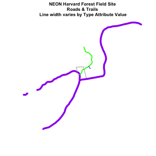
Plot Data
In the Explore Shapefile Attributes & Plot Shapefile Objects by Attribute Value in R tutorial we created a plot where we customized the width of each line in a spatial object according to a factor level or category. To do this, we create a vector of colors containing a color value for EACH feature in our spatial object grouped by factor level or category.
# view the factor levels
levels(lines_HARV$TYPE)

## [1] "boardwalk"  "footpath"   "stone wall" "woods road"

# create vector of line width values
lineWidth <- c(2,4,3,8)[lines_HARV$TYPE]
# view vector
lineWidth

##  [1] 8 4 4 3 3 3 3 3 3 2 8 8 8

# create a color palette of 4 colors - one for each factor level
roadPalette <- c("blue","green","grey","purple")
roadPalette

## [1] "blue"   "green"  "grey"   "purple"

# create a vector of colors - one for each feature in our vector object
# according to its attribute value
roadColors <- c("blue","green","grey","purple")[lines_HARV$TYPE]
roadColors

##  [1] "purple" "green"  "green"  "grey"   "grey"   "grey"   "grey"
##  [8] "grey"   "grey"   "blue"   "purple" "purple" "purple"

# create vector of line width values
lineWidth <- c(2,4,3,8)[lines_HARV$TYPE]
# view vector
lineWidth

##  [1] 8 4 4 3 3 3 3 3 3 2 8 8 8

# in this case, boardwalk (the first level) is the widest.
plot(lines_HARV,
     col=roadColors,
     main="NEON Harvard Forest Field Site\n Roads & Trails \nLine Width Varies by Type Attribute Value",
     lwd=lineWidth)
Add Plot Legend
In the the previous tutorial, we also learned how to add a basic legend to our plot.
-
bottomright: We specify the location of our legend by using a default keyword. We could also usetop,topright, etc. -
levels(objectName$attributeName): Label the legend elements using the categories oflevelsin an attribute (e.g., levels(lines_HARV$TYPE) means use the levels boardwalk, footpath, etc). -
fill=: apply unique colors to the boxes in our legend.palette()is the default set of colors that R applies to all plots.
Let's add a legend to our plot.
plot(lines_HARV,
     col=roadColors,
     main="NEON Harvard Forest Field Site\n Roads & Trails\n Default Legend")

# we can use the color object that we created above to color the legend objects
roadPalette

## [1] "blue"   "green"  "grey"   "purple"

# add a legend to our map
legend("bottomright",
       legend=levels(lines_HARV$TYPE),
       fill=roadPalette,
       bty="n", # turn off the legend border
       cex=.8) # decrease the font / legend size

However, what if we want to create a more complex plot with many shapefiles and unique symbols that need to be represented clearly in a legend?
Plot Multiple Vector Layers
Now, let's create a plot that combines our tower location (point_HARV),
site boundary (aoiBoundary_HARV) and roads (lines_HARV) spatial objects. We
will need to build a custom legend as well.
To begin, create a plot with the site boundary as the first layer. Then layer
the tower location and road data on top using add=TRUE.
# Plot multiple shapefiles
plot(aoiBoundary_HARV,
     col = "grey93",
     border="grey",
     main="NEON Harvard Forest Field Site")

plot(lines_HARV,
     col=roadColors,
     add = TRUE)

plot(point_HARV,
     add  = TRUE,
     pch = 19,
     col = "purple")
# assign plot to an object for easy modification!
plot_HARV<- recordPlot()
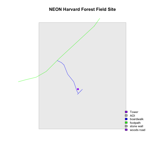
Customize Your Legend
Next, let's build a custom legend using the symbology (the colors and symbols) that we used to create the plot above. To do this, we will need to build three things:
- A list of all "labels" (the text used to describe each element in the legend to use in the legend.
- A list of colors used to color each feature in our plot.
- A list of symbols to use in the plot. NOTE: we have a combination of points, lines and polygons in our plot. So we will need to customize our symbols!
Let's create objects for the labels, colors and symbols so we can easily reuse them. We will start with the labels.
# create a list of all labels
labels <- c("Tower", "AOI", levels(lines_HARV$TYPE))
labels

## [1] "Tower"      "AOI"        "boardwalk"  "footpath"   "stone wall"
## [6] "woods road"

# render plot
plot_HARV

# add a legend to our map
legend("bottomright",
       legend=labels,
       bty="n", # turn off the legend border
       cex=.8) # decrease the font / legend size
Now we have a legend with the labels identified. Let's add colors to each legend element next. We can use the vectors of colors that we created earlier to do this.
# we have a list of colors that we used above - we can use it in the legend
roadPalette

## [1] "blue"   "green"  "grey"   "purple"

# create a list of colors to use
plotColors <- c("purple", "grey", roadPalette)
plotColors

## [1] "purple" "grey"   "blue"   "green"  "grey"   "purple"

# render plot
plot_HARV

# add a legend to our map
legend("bottomright",
       legend=labels,
       fill=plotColors,
       bty="n", # turn off the legend border
       cex=.8) # decrease the font / legend size
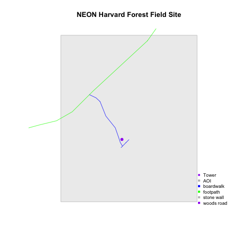
Great, now we have a legend! However, this legend uses boxes to symbolize each
element in the plot. It might be better if the lines were symbolized as a line
and the points were symbolized as a point symbol. We can customize this using
pch= in our legend: 16 is a point symbol, 15 is a box.
# create a list of pch values
# these are the symbols that will be used for each legend value
# ?pch will provide more information on values
plotSym <- c(16,15,15,15,15,15)
plotSym

## [1] 16 15 15 15 15 15

# Plot multiple shapefiles
plot_HARV

# to create a custom legend, we need to fake it
legend("bottomright",
       legend=labels,
       pch=plotSym,
       bty="n",
       col=plotColors,
       cex=.8)
Now we've added a point symbol to represent our point element in the plot. However
it might be more useful to use line symbols in our legend
rather than squares to represent the line data. We can create line symbols,
using lty = (). We have a total of 6 elements in our legend:
- A Tower Location
- An Area of Interest (AOI)
- and 4 Road types (levels)
The lty list designates, in order, which of those elements should be
designated as a line (1) and which should be designated as a symbol (NA).
Our object will thus look like lty = c(NA,NA,1,1,1,1). This tells R to only use a
line element for the 3-6 elements in our legend.
Once we do this, we still need to modify our pch element. Each line element
(3-6) should be represented by a NA value - this tells R to not use a
symbol, but to instead use a line.
# create line object
lineLegend = c(NA,NA,1,1,1,1)
lineLegend

## [1] NA NA  1  1  1  1

plotSym <- c(16,15,NA,NA,NA,NA)
plotSym

## [1] 16 15 NA NA NA NA

# plot multiple shapefiles
plot_HARV

# build a custom legend
legend("bottomright",
       legend=labels,
       lty = lineLegend,
       pch=plotSym,
       bty="n",
       col=plotColors,
       cex=.8)
![Roads and tower location at NEON Harvard Forest Field Site with color and a modified legend varied by attribute type; each symbol on the legend corresponds to the shapefile type [i.e., tower = point, roads = lines].](https://raw.githubusercontent.com/NEONScience/NEON-Data-Skills/main/tutorials/R/Geospatial-skills/intro-vector-r/02-plot-multiple-shapefiles-custom-legend/rfigs/refine-legend-1.png)
-
Using the
NEON-DS-Site-Layout-Files/HARV/PlotLocations_HARV.shpshapefile, create a map of study plot locations, with each point colored by the soil type (soilTypeOr). How many different soil types are there at this particular field site? Overlay this layer on top of thelines_HARVlayer (the roads). Create a custom legend that applies line symbols to lines and point symbols to the points. -
Modify the plot above. Tell R to plot each point, using a different symbol of
pchvalue. HINT: to do this, create a vector object of symbols by factor level using the syntax described above for line width:c(15,17)[lines_HARV$soilTypeOr]. Overlay this on top of the AOI Boundary. Create a custom legend.
![Roads and study plots at NEON Harvard Forest Field Site with color and a modified legend varied by attribute type; each symbol on the legend corresponds to the shapefile type [i.e., soil plots = points, roads = lines].](https://raw.githubusercontent.com/NEONScience/NEON-Data-Skills/main/tutorials/R/Geospatial-skills/intro-vector-r/02-plot-multiple-shapefiles-custom-legend/rfigs/challenge-code-plot-color-1.png)
![Roads and study plots at NEON Harvard Forest Field Site with color and a modified legend varied by attribute type; each symbol on the legend corresponds to the shapefile type [i.e., soil plots = points, roads = lines], and study plots symbols vary by soil type.](https://raw.githubusercontent.com/NEONScience/NEON-Data-Skills/main/tutorials/R/Geospatial-skills/intro-vector-r/02-plot-multiple-shapefiles-custom-legend/rfigs/challenge-code-plot-color-2.png)
Get Lesson Code
Vector 03: When Vector Data Don't Line Up - Handling Spatial Projection & CRS in R
Last Updated: Apr 8, 2021
In this tutorial, we will create a base map of our study site using a United States
state and country boundary accessed from the
.
We will learn how to map vector data that are in different CRS and thus
don't line up on a map.
Learning Objectives
After completing this tutorial, you will be able to:
- Identify the
CRSof a spatial dataset. - Differentiate between with geographic vs. projected coordinate reference systems.
- Use the
proj4string format which is one format used used to store & reference theCRSof a spatial object.
Things You’ll Need To Complete This Tutorial
You will need the most current version of R and, preferably, RStudio loaded
on your computer to complete this tutorial.
Install R Packages
-
raster:
install.packages("raster") -
rgdal:
install.packages("rgdal") -
sp:
install.packages("sp") -
More on Packages in R � Adapted from Software Carpentry.
Data to Download
These vector data provide information on the site characterization and infrastructure at the National Ecological Observatory Network's Harvard Forest field site. The Harvard Forest shapefiles are from the archives. US Country and State Boundary layers are from the .
The LiDAR and imagery data used to create this raster teaching data subset were collected over the National Ecological Observatory Network's Harvard Forest and San Joaquin Experimental Range field sites and processed at NEON headquarters. The entire dataset can be accessed by request from the .
Set Working Directory: This lesson assumes that you have set your working directory to the location of the downloaded and unzipped data subsets.
An overview of setting the working directory in R can be found here.
R Script & Challenge Code: NEON data lessons often contain challenges that reinforce learned skills. If available, the code for challenge solutions is found in the downloadable R script of the entire lesson, available in the footer of each lesson page.
Working With Spatial Data From Different Sources
To support a project, we often need to gather spatial datasets for from
different sources and/or data that cover different spatial extents. Spatial
data from different sources and that cover different extents are often in
different Coordinate Reference Systems (CRS).
Some reasons for data being in different CRS include:
- The data are stored in a particular CRS convention used by the data provider; perhaps a federal agency or a state planning office.
- The data are stored in a particular CRS that is customized to a region. For instance, many states prefer to use a State Plane projection customized for that state.
Check out this short video from highlighting how map projections can make continents seems proportionally larger or smaller than they actually are!
In this tutorial we will learn how to identify and manage spatial data
in different projections. We will learn how to reproject the data so that they
are in the same projection to support plotting / mapping. Note that these skills
are also required for any geoprocessing / spatial analysis, as data need to be in
the same CRS to ensure accurate results.
We will use the rgdal and raster libraries in this tutorial.
# load packages
library(rgdal)  # for vector work; sp package should always load with rgdal.
library (raster)   # for metadata/attributes- vectors or rasters

# set working directory to data folder
# setwd("pathToDirHere")
Import US Boundaries - Census Data
There are many good sources of boundary base layers that we can use to create a basemap. Some R packages even have these base layers built in to support quick and efficient mapping. In this tutorial, we will use boundary layers for the United States, provided by the
It is useful to have shapefiles to work with because we can add additional attributes to them if need be - for project specific mapping.
Read US Boundary File
We will use the readOGR() function to import the
/US-Boundary-Layers/US-State-Boundaries-Census-2014 layer into R. This layer
contains the boundaries of all continental states in the U.S.. Please note that
these data have been modified and reprojected from the original data downloaded
from the Census website to support the learning goals of this tutorial.
# Read the .csv file
State.Boundary.US <- readOGR("NEON-DS-Site-Layout-Files/US-Boundary-Layers",
          "US-State-Boundaries-Census-2014")

## OGR data source with driver: ESRI Shapefile
## Source: "/Users/olearyd/Git/data/NEON-DS-Site-Layout-Files/US-Boundary-Layers", layer: "US-State-Boundaries-Census-2014"
## with 58 features
## It has 10 fields
## Integer64 fields read as strings:  ALAND AWATER

## Warning in readOGR("NEON-DS-Site-Layout-Files/US-Boundary-Layers", "US-
## State-Boundaries-Census-2014"): Z-dimension discarded

# look at the data structure
class(State.Boundary.US)

## [1] "SpatialPolygonsDataFrame"
## attr(,"package")
## [1] "sp"
Note: the Z-dimension warning is normal. The readOGR() function doesn't import
z (vertical dimension or height) data by default. This is because not all
shapefiles contain z dimension data.
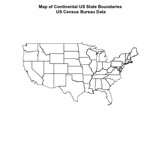
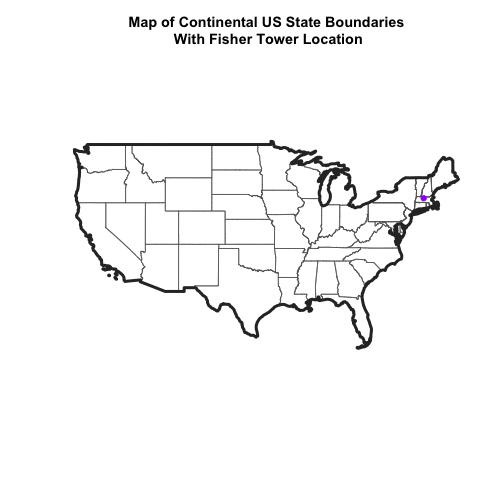
Now, let's plot the U.S. states data.
# view column names
plot(State.Boundary.US,
     main="Map of Continental US State Boundaries\n US Census Bureau Data")
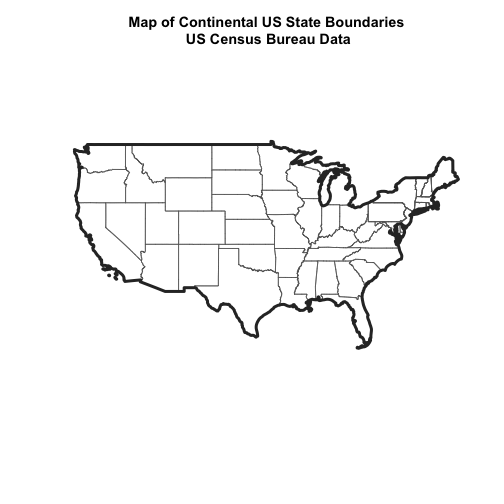
U.S. Boundary Layer
We can add a boundary layer of the United States to our map to make it look
nicer. We will import
NEON-DS-Site-Layout-Files/US-Boundary-Layers/US-Boundary-Dissolved-States.
If we specify a thicker line width using lwd=4 for the border layer, it will
make our map pop!
# Read the .csv file
Country.Boundary.US <- readOGR("NEON-DS-Site-Layout-Files/US-Boundary-Layers",
          "US-Boundary-Dissolved-States")

## OGR data source with driver: ESRI Shapefile
## Source: "/Users/olearyd/Git/data/NEON-DS-Site-Layout-Files/US-Boundary-Layers", layer: "US-Boundary-Dissolved-States"
## with 1 features
## It has 9 fields
## Integer64 fields read as strings:  ALAND AWATER

## Warning in readOGR("NEON-DS-Site-Layout-Files/US-Boundary-Layers", "US-
## Boundary-Dissolved-States"): Z-dimension discarded

# look at the data structure
class(Country.Boundary.US)

## [1] "SpatialPolygonsDataFrame"
## attr(,"package")
## [1] "sp"

# view column names
plot(State.Boundary.US,
     main="Map of Continental US State Boundaries\n US Census Bureau Data",
     border="gray40")

# view column names
plot(Country.Boundary.US,
     lwd=4,
     border="gray18",
     add=TRUE)
Next, let's add the location of a flux tower where our study area is. As we are adding these layers, take note of the class of each object.
# Import a point shapefile
point_HARV <- readOGR("NEON-DS-Site-Layout-Files/HARV/",
                      "HARVtower_UTM18N")

## OGR data source with driver: ESRI Shapefile
## Source: "/Users/olearyd/Git/data/NEON-DS-Site-Layout-Files/HARV", layer: "HARVtower_UTM18N"
## with 1 features
## It has 14 fields

class(point_HARV)

## [1] "SpatialPointsDataFrame"
## attr(,"package")
## [1] "sp"

# plot point - looks ok?
plot(point_HARV,
     pch = 19,
     col = "purple",
     main="Harvard Fisher Tower Location")
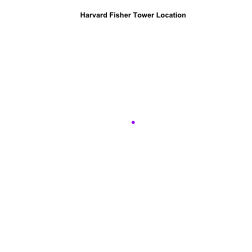
The plot above demonstrates that the tower point location data are readable and will plot! Let's next add it as a layer on top of the U.S. states and boundary layers in our basemap plot.
# plot state boundaries
plot(State.Boundary.US,
     main="Map of Continental US State Boundaries \n with Tower Location",
     border="gray40")

# add US border outline
plot(Country.Boundary.US,
     lwd=4,
     border="gray18",
     add=TRUE)

# add point tower location
plot(point_HARV,
     pch = 19,
     col = "purple",
     add=TRUE)
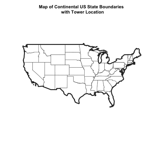
What do you notice about the resultant plot? Do you see the tower location in purple in the Massachusetts area? No! So what went wrong?
Let's check out the CRS (crs()) of both datasets to see if we can identify any
issues that might cause the point location to not plot properly on top of our
U.S. boundary layers.
# view CRS of our site data
crs(point_HARV)

## CRS arguments:
##  +proj=utm +zone=18 +datum=WGS84 +units=m +no_defs

# view crs of census data
crs(State.Boundary.US)

## CRS arguments: +proj=longlat +datum=WGS84 +no_defs

crs(Country.Boundary.US)

## CRS arguments: +proj=longlat +datum=WGS84 +no_defs
It looks like our data are in different CRS. We can tell this by looking at
the CRS strings in proj4 format.
Understanding CRS in Proj4 Format
The CRS for our data are given to us by R in proj4 format. Let's break
down the pieces of proj4 string. The string contains all of the individual
CRS elements that R or another GIS might need. Each element is specified
with a + sign, similar to how a .csv file is delimited or broken up by
a ,. After each + we see the CRS element being defined. For example
projection (proj=) and datum (datum=).
UTM Proj4 String
Our project string for point_HARV specifies the UTM projection as follows:
+proj=utm +zone=18 +datum=WGS84 +units=m +no_defs +ellps=WGS84 +towgs84=0,0,0
- proj=utm: the projection is UTM
- zone=18: the zone is 18
- datum=WGS84: the datum WGS84 (the datum refers to the 0,0 reference for the coordinate system used in the projection)
- units=m: the units for the coordinates are in METERS
- ellps=WGS84: the ellipsoid (how the earth's roundness is calculated) for the data is WGS84
Note that the zone is unique to the UTM projection. Not all CRS will have a
zone.
Geographic (lat / long) Proj4 String
Our project string for State.boundary.US and Country.boundary.US specifies
the lat/long projection as follows:
+proj=longlat +datum=WGS84 +no_defs +ellps=WGS84 +towgs84=0,0,0
- proj=longlat: the data are in a geographic (latitude and longitude) coordinate system
- datum=WGS84: the datum is WGS84
- ellps=WGS84: the ellipsoid is WGS84
Note that there are no specified units above. This is because this geographic coordinate reference system is in latitude and longitude which is most often recorded in Decimal Degrees.
CRS Units - View Object Extent
Next, let's view the extent or spatial coverage for the point_HARV spatial
object compared to the State.Boundary.US object.
# extent for HARV in UTM
extent(point_HARV)

## class      : Extent
## xmin       : 732183.2
## xmax       : 732183.2
## ymin       : 4713265
## ymax       : 4713265

# extent for object in geographic
extent(State.Boundary.US)

## class      : Extent
## xmin       : -124.7258
## xmax       : -66.94989
## ymin       : 24.49813
## ymax       : 49.38436
Note the difference in the units for each object. The extent for
State.Boundary.US is in latitude and longitude, which yields smaller numbers
representing decimal degree units; however, our tower location point
is in UTM, which is represented in meters.
Proj4 & CRS Resources
- To view a list of datum conversion factors, type
projInfo(type = "datum")into the R console.
Reproject Vector Data
Now we know our data are in different CRS. To address this, we have to modify
or reproject the data so they are all in the same CRS. We can use
spTransform() function to reproject our data. When we reproject the data, we
specify the CRS that we wish to transform our data to. This CRS contains
the datum, units and other information that R needs to reproject our data.
The spTransform() function requires two inputs:
- The name of the object that you wish to transform
- The CRS that you wish to transform that object too. In this case we can
use the
crs()of theState.Boundary.USobject as follows:crs(State.Boundary.US)
Next, let's reproject our point layer into the geographic latitude and
longitude WGS84 coordinate reference system (CRS).
# reproject data
point_HARV_WGS84 <- spTransform(point_HARV,
                                crs(State.Boundary.US))

# what is the CRS of the new object
crs(point_HARV_WGS84)

## CRS arguments: +proj=longlat +datum=WGS84 +no_defs

# does the extent look like decimal degrees?
extent(point_HARV_WGS84)

## class      : Extent
## xmin       : -72.17266
## xmax       : -72.17266
## ymin       : 42.5369
## ymax       : 42.5369
Once our data are reprojected, we can try to plot again.
# plot state boundaries
plot(State.Boundary.US,
     main="Map of Continental US State Boundaries\n With Fisher Tower Location",
     border="gray40")

# add US border outline
plot(Country.Boundary.US,
     lwd=4,
     border="gray18",
     add=TRUE)

# add point tower location
plot(point_HARV_WGS84,
     pch = 19,
     col = "purple",
     add=TRUE)
Reprojecting our data ensured that things line up on our map! It will also allow us to perform any required geoprocessing (spatial calculations / transformations) on our data.
Create a map of the North Eastern United States as follows:
- Import and plot
Boundary-US-State-NEast.shp. Adjust line width as necessary. - Reproject the layer into UTM zone 18 north.
- Layer the Fisher Tower point location
point_HARVon top of the above plot. - Add a title to your plot.
- Add a legend to your plot that shows both the state boundary (line) and the Tower location point.
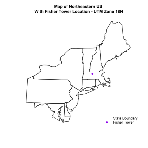
Get Lesson Code
Vector 04: Convert from .csv to a Shapefile in R
Last Updated: Apr 8, 2021
This tutorial will review how to import spatial points stored in .csv (Comma
Separated Value) format into
R as a spatial object - a SpatialPointsDataFrame. We will also
reproject data imported in a shapefile format, export a shapefile from an
R spatial object, and plot raster and vector data as
layers in the same plot.
Learning Objectives
After completing this tutorial, you will be able to:
- Import .csv files containing x,y coordinate locations into R.
- Convert a .csv to a spatial object.
- Project coordinate locations provided in a Geographic Coordinate System (Latitude, Longitude) to a projected coordinate system (UTM).
- Plot raster and vector data in the same plot to create a map.
Things You’ll Need To Complete This Tutorial
You will need the most current version of R and, preferably, RStudio loaded
on your computer to complete this tutorial.
Install R Packages
-
raster:
install.packages("raster") -
rgdal:
install.packages("rgdal") -
sp:
install.packages("sp") -
More on Packages in R � Adapted from Software Carpentry.
Data to Download
These vector data provide information on the site characterization and infrastructure at the National Ecological Observatory Network's Harvard Forest field site. The Harvard Forest shapefiles are from the archives. US Country and State Boundary layers are from the .
The LiDAR and imagery data used to create this raster teaching data subset were collected over the National Ecological Observatory Network's Harvard Forest and San Joaquin Experimental Range field sites and processed at NEON headquarters. The entire dataset can be accessed by request from the .
Set Working Directory: This lesson assumes that you have set your working directory to the location of the downloaded and unzipped data subsets.
An overview of setting the working directory in R can be found here.
R Script & Challenge Code: NEON data lessons often contain challenges that reinforce learned skills. If available, the code for challenge solutions is found in the downloadable R script of the entire lesson, available in the footer of each lesson page.
Spatial Data in Text Format
The HARV_PlotLocations.csv file contains x, y (point) locations for study
plots where NEON collects data on
vegetation and other ecological metrics.
We would like to:
- Create a map of these plot locations.
- Export the data in a
shapefileformat to share with our colleagues. This shapefile can be imported into any GIS software. - Create a map showing vegetation height with plot locations layered on top.
Spatial data are sometimes stored in a text file format (.txt or .csv). If
the text file has an associated x and y location column, then we can
convert it into an R spatial object, which, in the case of point data,
will be a SpatialPointsDataFrame. The SpatialPointsDataFrame
allows us to store both the x,y values that represent the coordinate location
of each point and the associated attribute data, or columns describing each
feature in the spatial object.
We will use the rgdal and raster libraries in this tutorial.
# load packages
library(rgdal)  # for vector work; sp package should always load with rgdal
library (raster)   # for metadata/attributes- vectors or rasters

# set working directory to data folder
# setwd("pathToDirHere")
Import .csv
To begin let's import the .csv file that contains plot coordinate x, y
locations at the NEON Harvard Forest Field Site (HARV_PlotLocations.csv) into
R. Note that we set stringsAsFactors=FALSE so our data imports as a
character rather than a factor class.
# Read the .csv file
plot.locations_HARV <-
  read.csv("NEON-DS-Site-Layout-Files/HARV/HARV_PlotLocations.csv",
           stringsAsFactors = FALSE)

# look at the data structure
str(plot.locations_HARV)

## 'data.frame':	21 obs. of  16 variables:
##  $ easting   : num  731405 731934 731754 731724 732125 ...
##  $ northing  : num  4713456 4713415 4713115 4713595 4713846 ...
##  $ geodeticDa: chr  "WGS84" "WGS84" "WGS84" "WGS84" ...
##  $ utmZone   : chr  "18N" "18N" "18N" "18N" ...
##  $ plotID    : chr  "HARV_015" "HARV_033" "HARV_034" "HARV_035" ...
##  $ stateProvi: chr  "MA" "MA" "MA" "MA" ...
##  $ county    : chr  "Worcester" "Worcester" "Worcester" "Worcester" ...
##  $ domainName: chr  "Northeast" "Northeast" "Northeast" "Northeast" ...
##  $ domainID  : chr  "D01" "D01" "D01" "D01" ...
##  $ siteID    : chr  "HARV" "HARV" "HARV" "HARV" ...
##  $ plotType  : chr  "distributed" "tower" "tower" "tower" ...
##  $ subtype   : chr  "basePlot" "basePlot" "basePlot" "basePlot" ...
##  $ plotSize  : int  1600 1600 1600 1600 1600 1600 1600 1600 1600 1600 ...
##  $ elevation : num  332 342 348 334 353 ...
##  $ soilTypeOr: chr  "Inceptisols" "Inceptisols" "Inceptisols" "Histosols" ...
##  $ plotdim_m : int  40 40 40 40 40 40 40 40 40 40 ...
Also note that plot.locations_HARV is a data.frame that contains 21
locations (rows) and 15 variables (attributes).
Next, let's explore data.frame to determine whether it contains
columns with coordinate values. If we are lucky, our .csv will contain columns
labeled:
- "X" and "Y" OR
- Latitude and Longitude OR
- easting and northing (UTM coordinates)
Let's check out the column names of our file to look for these.
# view column names
names(plot.locations_HARV)

##  [1] "easting"    "northing"   "geodeticDa" "utmZone"    "plotID"
##  [6] "stateProvi" "county"     "domainName" "domainID"   "siteID"
## [11] "plotType"   "subtype"    "plotSize"   "elevation"  "soilTypeOr"
## [16] "plotdim_m"
Identify X,Y Location Columns
View the column names, we can see that our data.frame that contains several
fields that might contain spatial information. The plot.locations_HARV$easting
and plot.locations_HARV$northing columns contain these coordinate values.
# view first 6 rows of the X and Y columns
head(plot.locations_HARV$easting)

## [1] 731405.3 731934.3 731754.3 731724.3 732125.3 731634.3

head(plot.locations_HARV$northing)

## [1] 4713456 4713415 4713115 4713595 4713846 4713295

# note that  you can also call the same two columns using their COLUMN NUMBER
# view first 6 rows of the X and Y columns
head(plot.locations_HARV[,1])

## [1] 731405.3 731934.3 731754.3 731724.3 732125.3 731634.3

head(plot.locations_HARV[,2])

## [1] 4713456 4713415 4713115 4713595 4713846 4713295
So, we have coordinate values in our data.frame but in order to convert our
data.frame to a SpatialPointsDataFrame, we also need to know the CRS
associated with these coordinate values.
There are several ways to figure out the CRS of spatial data in text format.
- We can check the file metadata in hopes that the CRS was recorded in the data. For more information on metadata, check out the Why Metadata Are Important: How to Work with Metadata in Text & EML Format tutorial.
- We can explore the file itself to see if CRS information is embedded in the file header or somewhere in the data columns.
Following the easting and northing columns, there is a geodeticDa and a
utmZone column. These appear to contain CRS information
(datum and projection), so let's view those next.
# view first 6 rows of the X and Y columns
head(plot.locations_HARV$geodeticDa)

## [1] "WGS84" "WGS84" "WGS84" "WGS84" "WGS84" "WGS84"

head(plot.locations_HARV$utmZone)

## [1] "18N" "18N" "18N" "18N" "18N" "18N"
It is not typical to store CRS information in a column, but this particular
file contains CRS information this way. The geodeticDa and utmZone columns
contain the information that helps us determine the CRS:
-
geodeticDa: WGS84 -- this is geodetic datum WGS84 -
utmZone: 18
In
When Vector Data Don't Line Up - Handling Spatial Projection & CRS in R tutorial
we learned about the components of a proj4 string. We have everything we need
to now assign a CRS to our data.frame.
To create the proj4 associated with UTM Zone 18 WGS84 we could look up the
projection on the
which contains a list of CRS formats for each projection:
- This link shows .
However, if we have other data in the UTM Zone 18N projection, it's much
easier to simply assign the crs() in proj4 format from that object to our
new spatial object. Let's import the roads layer from Harvard forest and check
out its CRS.
Note: if you do not have a CRS to borrow from another raster, see Option 2 in the next section for how to convert to a spatial object and assign a CRS.
# Import the line shapefile
lines_HARV <- readOGR( "NEON-DS-Site-Layout-Files/HARV/", "HARV_roads")

## OGR data source with driver: ESRI Shapefile
## Source: "/Users/olearyd/Git/data/NEON-DS-Site-Layout-Files/HARV", layer: "HARV_roads"
## with 13 features
## It has 15 fields

# view CRS
crs(lines_HARV)

## CRS arguments:
##  +proj=utm +zone=18 +datum=WGS84 +units=m +no_defs

# view extent
extent(lines_HARV)

## class      : Extent
## xmin       : 730741.2
## xmax       : 733295.5
## ymin       : 4711942
## ymax       : 4714260
Exploring the data above, we can see that the lines shapefile is in
UTM zone 18N. We can thus use the CRS from that spatial object to convert our
non-spatial data.frame into a spatialPointsDataFrame.
Next, let's create a crs object that we can use to define the CRS of our
SpatialPointsDataFrame when we create it.
# create crs object
utm18nCRS <- crs(lines_HARV)
utm18nCRS

## CRS arguments:
##  +proj=utm +zone=18 +datum=WGS84 +units=m +no_defs

class(utm18nCRS)

## [1] "CRS"
## attr(,"package")
## [1] "sp"
.csv to R SpatialPointsDataFrame
Let's convert our data.frame into a SpatialPointsDataFrame. To do
this, we need to specify:
- The columns containing X (
easting) and Y (northing) coordinate values - The CRS that the column coordinate represent (units are included in the CRS).
- Optional: the other columns stored in the data frame that you wish to append as attributes to your spatial object.
We can add the CRS in two ways; borrow the CRS from another raster that
already has it assigned (Option 1) or to add it directly using the proj4string
(Option 2).
Option 1: Borrow CRS
We will use the SpatialPointsDataFrame() function to perform the conversion
and add the CRS from our utm18nCRS object.
# note that the easting and northing columns are in columns 1 and 2
plot.locationsSp_HARV <- SpatialPointsDataFrame(plot.locations_HARV[,1:2],
                    plot.locations_HARV,    #the R object to convert
                    proj4string = utm18nCRS)   # assign a CRS

# look at CRS
crs(plot.locationsSp_HARV)

## CRS arguments:
##  +proj=utm +zone=18 +datum=WGS84 +units=m +no_defs
Option 2: Assigning CRS
If we didn't have a raster from which to borrow the CRS, we can directly assign it using either of two equivalent, but slightly different syntaxes.
# first, convert the data.frame to spdf
r <- SpatialPointsDataFrame(plot.locations_HARV[,1:2],
                    plot.locations_HARV)

# second, assign the CRS in one of two ways
r <- crs("+proj=utm +zone=18 +datum=WGS84 +units=m +no_defs
				 +ellps=WGS84 +towgs84=0,0,0" )
# or

crs(r) <- "+proj=utm +zone=18 +datum=WGS84 +units=m +no_defs
				 +ellps=WGS84 +towgs84=0,0,0"
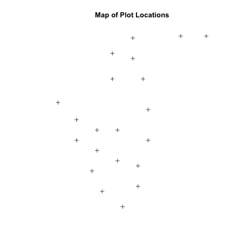
Plot Spatial Object
We now have a spatial R object, we can plot our newly created spatial object.
# plot spatial object
plot(plot.locationsSp_HARV,
     main="Map of Plot Locations")
Define Plot Extent
In
Open and Plot Shapefiles in R
we learned about spatial object extent. When we plot several spatial layers in
R, the first layer that is plotted becomes the extent of the plot. If we add
additional layers that are outside of that extent, then the data will not be
visible in our plot. It is thus useful to know how to set the spatial extent of
a plot using xlim and ylim.
Let's first create a SpatialPolygon object from the
NEON-DS-Site-Layout-Files/HarClip_UTMZ18 shapefile. (If you have completed
Vector 00-02 tutorials in this
Introduction to Working with Vector Data in R
series, you can skip this code as you have already created this object.)
# create boundary object
aoiBoundary_HARV <- readOGR("NEON-DS-Site-Layout-Files/HARV/",
                            "HarClip_UTMZ18")

## OGR data source with driver: ESRI Shapefile
## Source: "/Users/olearyd/Git/data/NEON-DS-Site-Layout-Files/HARV", layer: "HarClip_UTMZ18"
## with 1 features
## It has 1 fields
## Integer64 fields read as strings:  id
To begin, let's plot our aoiBoundary object with our vegetation plots.
# plot Boundary
plot(aoiBoundary_HARV,
     main="AOI Boundary\nNEON Harvard Forest Field Site")

# add plot locations
plot(plot.locationsSp_HARV,
     pch=8, add=TRUE)
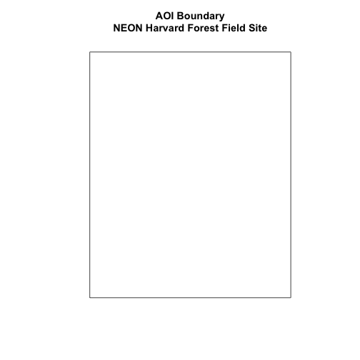
# no plots added, why? CRS?
# view CRS of each
crs(aoiBoundary_HARV)

## CRS arguments:
##  +proj=utm +zone=18 +datum=WGS84 +units=m +no_defs

crs(plot.locationsSp_HARV)

## CRS arguments:
##  +proj=utm +zone=18 +datum=WGS84 +units=m +no_defs
When we attempt to plot the two layers together, we can see that the plot locations are not rendered. Our data are in the same projection, so what is going on?
# view extent of each
extent(aoiBoundary_HARV)

## class      : Extent
## xmin       : 732128
## xmax       : 732251.1
## ymin       : 4713209
## ymax       : 4713359

extent(plot.locationsSp_HARV)

## class      : Extent
## xmin       : 731405.3
## xmax       : 732275.3
## ymin       : 4712845
## ymax       : 4713846

# add extra space to right of plot area;
# par(mar=c(5.1, 4.1, 4.1, 8.1), xpd=TRUE)

plot(extent(plot.locationsSp_HARV),
     col="purple",
     xlab="easting",
     ylab="northing", lwd=8,
     main="Extent Boundary of Plot Locations \nCompared to the AOI Spatial Object",
     ylim=c(4712400,4714000)) # extent the y axis to make room for the legend

plot(extent(aoiBoundary_HARV),
     add=TRUE,
     lwd=6,
     col="springgreen")

legend("bottomright",
       #inset=c(-0.5,0),
       legend=c("Layer One Extent", "Layer Two Extent"),
       bty="n",
       col=c("purple","springgreen"),
       cex=.8,
       lty=c(1,1),
       lwd=6)
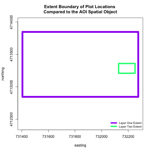
The extents of our two objects are different. plot.locationsSp_HARV is
much larger than aoiBoundary_HARV. When we plot aoiBoundary_HARV first, R
uses the extent of that object to as the plot extent. Thus the points in the
plot.locationsSp_HARV object are not rendered. To fix this, we can manually
assign the plot extent using xlims and ylims. We can grab the extent
values from the spatial object that has a larger extent. Let's try it.
plotLoc.extent <- extent(plot.locationsSp_HARV)
plotLoc.extent
## class : Extent
## xmin : 731405.3
## xmax : 732275.3
## ymin : 4712845
## ymax : 4713846
# grab the x and y min and max values from the spatial plot locations layer
xmin <- plotLoc.extent@xmin
xmax <- plotLoc.extent@xmax
ymin <- plotLoc.extent@ymin
ymax <- plotLoc.extent@ymax
# adjust the plot extent using x and ylim
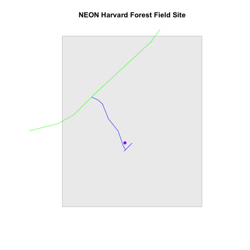
plot(aoiBoundary_HARV,
main="NEON Harvard Forest Field Site\nModified Extent",
border="darkgreen",
xlim=c(xmin,xmax),
ylim=c(ymin,ymax))
plot(plot.locationsSp_HARV,
pch=8,
col="purple",
add=TRUE)
# add a legend
legend("bottomright",
legend=c("Plots", "AOI Boundary"),
pch=c(8,NA),
lty=c(NA,1),
bty="n",
col=c("purple","darkgreen"),
cex=.8)
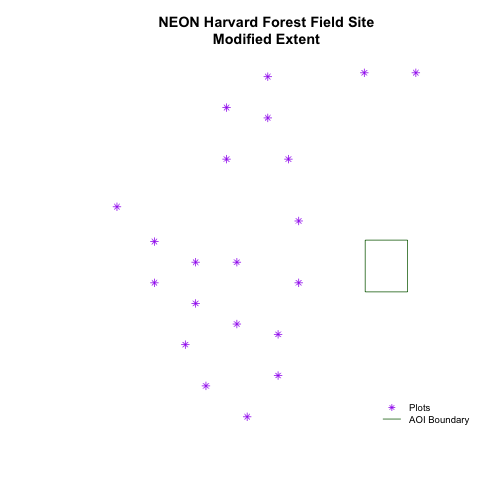
Import the .csv: HARV/HARV_2NewPhenPlots.csv into R and do the following:
- Find the X and Y coordinate locations. Which value is X and which value is Y?
- These data were collected in a geographic coordinate system (WGS84). Convert
the
data.frameinto an RspatialPointsDataFrame. - Plot the new points with the plot location points from above. Be sure to add a legend. Use a different symbol for the 2 new points! You may need to adjust the X and Y limits of your plot to ensure that both points are rendered by R!
If you have extra time, feel free to add roads and other layers to your map!
HINT: Refer to When Vector Data Don't Line Up - Handling Spatial Projection & CRS in R tutorial for more on working with geographic coordinate systems. You may want to "borrow" the projection from the objects used in that tutorial!
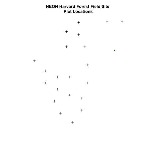
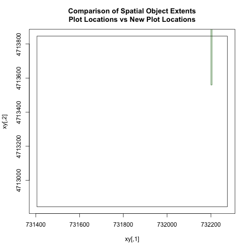
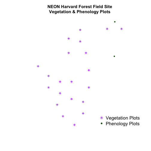
Export a Shapefile
We can write an R spatial object to a shapefile using the writeOGR function
in rgdal. To do this we need the following arguments:
- the name of the spatial object (
plot.locationsSp_HARV) - the directory where we want to save our shapefile
(to use
current = getwd()or you can specify a different path) - the name of the new shapefile (
PlotLocations_HARV) - the driver which specifies the file format (ESRI Shapefile)
We can now export the spatial object as a shapefile.
# write a shapefile
writeOGR(plot.locationsSp_HARV, getwd(),
         "PlotLocations_HARV", driver="ESRI Shapefile")
Get Lesson Code
Vector 05: Crop Raster Data and Extract Summary Pixels Values From Rasters in R
Last Updated: Apr 8, 2021
This tutorial explains how to crop a raster using the extent of a vector shapefile. We will also cover how to extract values from a raster that occur within a set of polygons, or in a buffer (surrounding) region around a set of points.
Learning Objectives
After completing this tutorial, you will be able to:
- Crop a raster to the extent of a vector layer.
- Extract values from raster that correspond to a vector file overlay.
Things You’ll Need To Complete This Tutorial
You will need the most current version of R and, preferably, RStudio loaded
on your computer to complete this tutorial.
Install R Packages
-
raster:
install.packages("raster") -
rgdal:
install.packages("rgdal") -
sp:
install.packages("sp") -
More on Packages in R � Adapted from Software Carpentry.
Download Data
These vector data provide information on the site characterization and infrastructure at the National Ecological Observatory Network's Harvard Forest field site. The Harvard Forest shapefiles are from the archives. US Country and State Boundary layers are from the .
The LiDAR and imagery data used to create this raster teaching data subset were collected over the National Ecological Observatory Network's Harvard Forest and San Joaquin Experimental Range field sites and processed at NEON headquarters. The entire dataset can be accessed by request from the .
Set Working Directory: This lesson assumes that you have set your working directory to the location of the downloaded and unzipped data subsets.
An overview of setting the working directory in R can be found here.
R Script & Challenge Code: NEON data lessons often contain challenges that reinforce learned skills. If available, the code for challenge solutions is found in the downloadable R script of the entire lesson, available in the footer of each lesson page.
Crop a Raster to Vector Extent
We often work with spatial layers that have different spatial extents.
The graphic below illustrates the extent of several of the spatial layers that we have worked with in this vector data tutorial series:
- Area of interest (AOI) -- blue
- Roads and trails -- purple
- Vegetation plot locations -- black
and a raster file, that we will introduce this tutorial:
- A canopy height model (CHM) in GeoTIFF format -- green
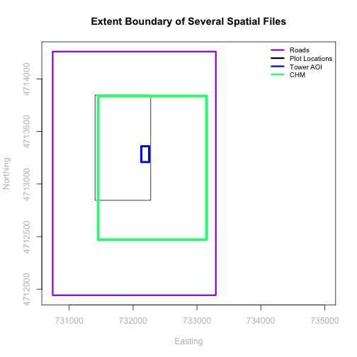
Frequent use cases of cropping a raster file include reducing file size and creating maps.
Sometimes we have a raster file that is much larger than our study area or area of interest. In this case, it is often most efficient to crop the raster to the extent of our study area to reduce file sizes as we process our data.
Cropping a raster can also be useful when creating visually appealing maps so that the raster layer matches the extent of the desired vector layers.
Import Data
We will begin by importing four vector shapefiles (field site boundary, roads/trails, tower location, and veg study plot locations) and one raster GeoTIFF file, a Canopy Height Model for the Harvard Forest, Massachusetts. These data can be used to create maps that characterize our study location.
If you have completed the Vector 00-04 tutorials in this Introduction to Working with Vector Data in R series, you can skip this code as you have already created these object.)
# load necessary packages
library(rgdal)  # for vector work; sp package should always load with rgdal.
library (raster)

# set working directory to data folder
# setwd("pathToDirHere")

# Imported in Vector 00: Vector Data in R - Open & Plot Data
# shapefile
aoiBoundary_HARV <- readOGR("NEON-DS-Site-Layout-Files/HARV/",
                            "HarClip_UTMZ18")
# Import a line shapefile
lines_HARV <- readOGR( "NEON-DS-Site-Layout-Files/HARV/",
                       "HARV_roads")
# Import a point shapefile
point_HARV <- readOGR("NEON-DS-Site-Layout-Files/HARV/",
                      "HARVtower_UTM18N")

# Imported in  Vector 02: .csv to Shapefile in R
# import raster Canopy Height Model (CHM)
chm_HARV <-
  raster("NEON-DS-Airborne-Remote-Sensing/HARV/CHM/HARV_chmCrop.tif")
Crop a Raster Using Vector Extent
We can use the crop function to crop a raster to the extent of another spatial
object. To do this, we need to specify the raster to be cropped and the spatial
object that will be used to crop the raster. R will use the extent of the
spatial object as the cropping boundary.
# plot full CHM
plot(chm_HARV,
     main="LiDAR CHM - Not Cropped\nNEON Harvard Forest Field Site")
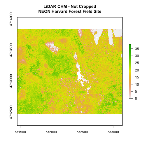
# crop the chm
chm_HARV_Crop <- crop(x = chm_HARV, y = aoiBoundary_HARV)

# plot full CHM
plot(extent(chm_HARV),
     lwd=4,col="springgreen",
     main="LiDAR CHM - Cropped\nNEON Harvard Forest Field Site",
     xlab="easting", ylab="northing")

plot(chm_HARV_Crop,
     add=TRUE)
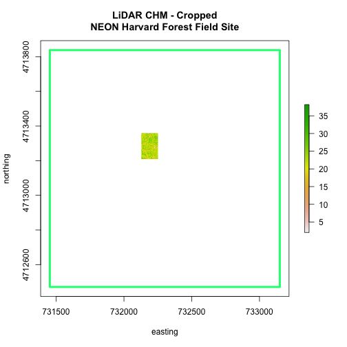
We can see from the plot above that the full CHM extent (plotted in green) is
much larger than the resulting cropped raster. Our new cropped CHM now has the
same extent as the aoiBoundary_HARV object that was used as a crop extent
(blue boarder below).
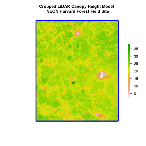
We can look at the extent of all the other objects.
# lets look at the extent of all of our objects
extent(chm_HARV)

## class      : Extent
## xmin       : 731453
## xmax       : 733150
## ymin       : 4712471
## ymax       : 4713838

extent(chm_HARV_Crop)

## class      : Extent
## xmin       : 732128
## xmax       : 732251
## ymin       : 4713209
## ymax       : 4713359

extent(aoiBoundary_HARV)

## class      : Extent
## xmin       : 732128
## xmax       : 732251.1
## ymin       : 4713209
## ymax       : 4713359
Which object has the largest extent? Our plot location extent is not the largest but it is larger than the AOI Boundary. It would be nice to see our vegetation plot locations with the Canopy Height Model information.
- Crop the Canopy Height Model to the extent of the study plot locations.
- Plot the vegetation plot location points on top of the Canopy Height Model.
If you completed the
.csv to Shapefile in R tutorial
you have these plot locations as the spatial R spatial object
plot.locationsSp_HARV. Otherwise, import the locations from the
\HARV\PlotLocations_HARV.shp shapefile in the downloaded data.
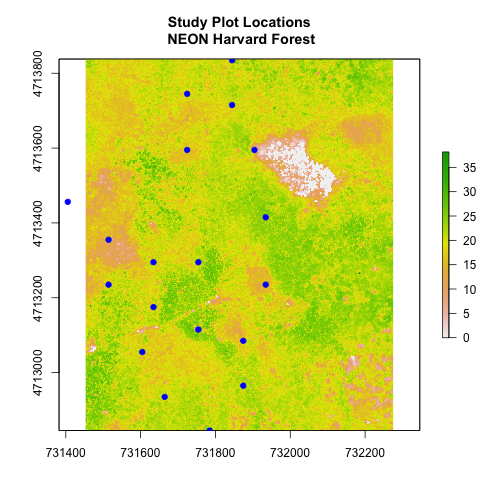
In the plot above, created in the challenge, all the vegetation plot locations (blue) appear on the Canopy Height Model raster layer except for one. One is situated on the white space. Why?
A modification of the first figure in this tutorial is below, showing the relative extents of all the spatial objects. Notice that the extent for our vegetation plot layer (black) extends further west than the extent of our CHM raster (bright green). The crop function will make a raster extent smaller, it will not expand the extent in areas where there are no data. Thus, extent of our vegetation plot layer will still extend further west than the extent of our (cropped) raster data (dark green).
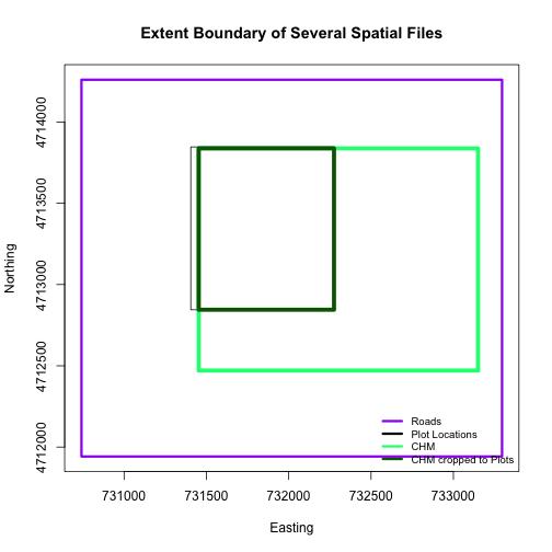
Define an Extent
We can also use an extent() method to define an extent to be used as a cropping
boundary. This creates an object of class extent.
# extent format (xmin,xmax,ymin,ymax)
new.extent <- extent(732161.2, 732238.7, 4713249, 4713333)
class(new.extent)

## [1] "Extent"
## attr(,"package")
## [1] "raster"
Once we have defined the extent, we can use the crop function to crop our
raster.
# crop raster
CHM_HARV_manualCrop <- crop(x = chm_HARV, y = new.extent)

# plot extent boundary and newly cropped raster
plot(aoiBoundary_HARV,
     main = "Manually Cropped Raster\n NEON Harvard Forest Field Site")
plot(new.extent,
     col="brown",
     lwd=4,
     add = TRUE)
plot(CHM_HARV_manualCrop,
     add = TRUE)
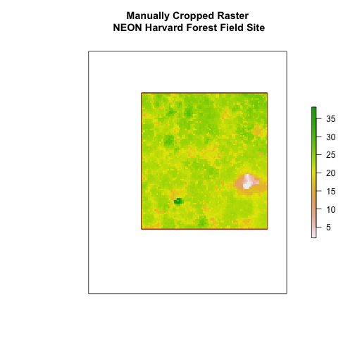
Notice that our manually set new.extent (in red) is smaller than the
aoiBoundary_HARV and that the raster is now the same as the new.extent
object.
See the documentation for the extent() function for more ways
to create an extent object using ??raster::extent
Extract Raster Pixels Values Using Vector Polygons
Often we want to extract values from a raster layer for particular locations - for example, plot locations that we are sampling on the ground.
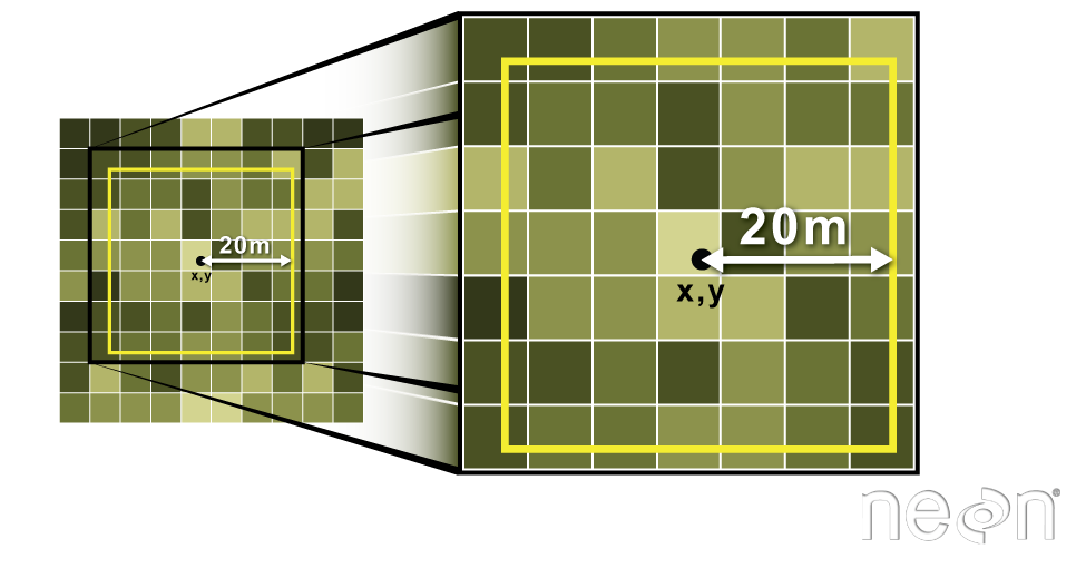
To do this in R, we use the extract() function. The extract() function
requires:
- The raster that we wish to extract values from
- The vector layer containing the polygons that we wish to use as a boundary or boundaries
NOTE: We can tell it to store the output values in a data.frame using
df=TRUE (optional, default is to NOT return a data.frame) .
We will begin by extracting all canopy height pixel values located within our
aoiBoundary polygon which surrounds the tower located at the NEON Harvard
Forest field site.
# extract tree height for AOI
# set df=TRUE to return a data.frame rather than a list of values
tree_height <- raster::extract(x = chm_HARV,
                       y = aoiBoundary_HARV,
                       df = TRUE)

# view the object
head(tree_height)

##   ID HARV_chmCrop
## 1  1        21.20
## 2  1        23.85
## 3  1        23.83
## 4  1        22.36
## 5  1        23.95
## 6  1        23.89

nrow(tree_height)

## [1] 18450
When we use the extract command, R extracts the value for each pixel located
within the boundary of the polygon being used to perform the extraction, in
this case the aoiBoundary object (1 single polygon). Using the aoiBoundary as the boundary polygon, the
function extracted values from 18,450 pixels.
The extract function returns a list of values as default, but you can tell R
to summarize the data in some way or to return the data as a data.frame
(df=TRUE).
We can create a histogram of tree height values within the boundary to better
understand the structure or height distribution of trees. We can also use the
summary() function to view descriptive statistics including min, max and mean
height values to help us better understand vegetation at our field
site.
# view histogram of tree heights in study area
hist(tree_height$HARV_chmCrop,
     main="Histogram of CHM Height Values (m) \nNEON Harvard Forest Field Site",
     col="springgreen",
     xlab="Tree Height", ylab="Frequency of Pixels")
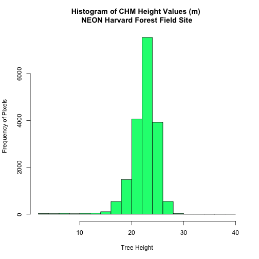
# view summary of values
summary(tree_height$HARV_chmCrop)

##    Min. 1st Qu.  Median    Mean 3rd Qu.    Max.
##    2.03   21.36   22.81   22.43   23.97   38.17
- Check out the documentation for the
extract()function for more details (??raster::extract).
Summarize Extracted Raster Values
We often want to extract summary values from a raster. We can tell R the type
of summary statistic we are interested in using the fun= method. Let's extract
a mean height value for our AOI.
# extract the average tree height (calculated using the raster pixels)
# located within the AOI polygon
av_tree_height_AOI <- raster::extract(x = chm_HARV,
                              y = aoiBoundary_HARV,
                              fun=mean,
                              df=TRUE)

# view output
av_tree_height_AOI

##   ID HARV_chmCrop
## 1  1     22.43018
It appears that the mean height value, extracted from our LiDAR data derived canopy height model is 22.43 meters.
Extract Data using x,y Locations
We can also extract pixel values from a raster by defining a buffer or area
surrounding individual point locations using the extract() function. To do this
we define the summary method (fun=mean) and the buffer distance (buffer=20)
which represents the radius of a circular region around each point.
The units of the buffer are the same units of the data CRS.
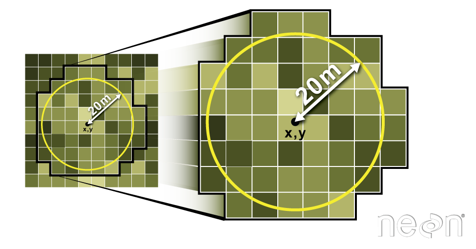
Let's put this into practice by figuring out the average tree height in the 20m around the tower location.
# what are the units of our buffer
crs(point_HARV)

## CRS arguments:
##  +proj=utm +zone=18 +datum=WGS84 +units=m +no_defs

# extract the average tree height (height is given by the raster pixel value)
# at the tower location
# use a buffer of 20 meters and mean function (fun)
av_tree_height_tower <- raster::extract(x = chm_HARV,
                                y = point_HARV,
                                buffer=20,
                                fun=mean,
                                df=TRUE)

# view data
head(av_tree_height_tower)

##   ID HARV_chmCrop
## 1  1     22.38812

# how many pixels were extracted
nrow(av_tree_height_tower)

## [1] 1
Use the plot location points shapefile HARV/plot.locations_HARV.shp or spatial
object plot.locationsSp_HARV to extract an average tree height value for the
area within 20m of each vegetation plot location in the study area.
Create a simple plot showing the mean tree height of each plot using the plot()
function in base-R.