AGÕæÈË°Ù¼ÒÀÖ¹Ù·½ÍøÕ¾

Setting up Jupyter Notebooks

You can set up your notebook in several ways. Here we present the Anaconda Python distribution method so as to follow the Data Institute set up instructions.

Browser

First, make sure you have an updated browser on which to run the app. Both Mozilla Firefox and Google Chrome work well.

Installation

Data Institute participants should have already installed Jupyter Notebooks through the Anaconda installation during the Data Institute set up instructions.

If you install Python using pip you can install the Jupyter package with the following code.

 
# Python2
pip install jupyter
# Python 3
pip3 install jupyter

Set up Environment

We need to set up the Python environment that we will be working in for the Notebook. This allows us to have different Python environments for different projects. The following directions pertain directly to the set up for the 2018 Data Institute on Remote Sensing with Reproducible Workflows, however, you can adapt them to the specific Python version and packages you wish to work with.

If you haven't yet created a Python 3.8 environment (released October 2019), you'll need to do that now. You can use the single line provided below, or refer back to the Python section of the installation instructions, for more details. To create this Python 3.8 environment, you must first install Anaconda Navigator onto your computer, then open the Anaconda Prompt application (or your terminal) and type the following into the prompt window:

conda create -n p38 python=3.8 anaconda

And activate the Python 3.8 environment:

On Mac:

source activate p38

On Windows:

activate p38

In the terminal application, navigate to the directory (cd) where you want the Jupyter Notebooks to be saved (or where they already exist).

Once here, we want to create a new Jupyter kernel for the Python 3.8 conda environment (p38) that we'll be using with Jupyter Notebooks.

With the p38 environment activated, in your Command Prompt/Terminal, type:

python -m ipykernel install --user --name p38 --display-name "Python 3.8 NEON-RSDI"

This command tells Python to create a new ipy (aka Jupyter Notebook) kernel using the Python environment we set up and called "p38". Then we tell it to use the display name for this new kernel as "Python 3.8 NEON-RSDI". You will use this name to identify the specific kernel you want to work with in the Notebook space, so name it descriptively, especially if you think you'll be using several different kernels.

Using Jupyter Notebooks

Launching the Application

To launch the application either launch it from the Anaconda Navigator or by typing jupyter notebook into your terminal or command window.

 
# Launch Jupyter
jupyter notebook

More information can be found in the Read the Docs .

Navigating the Jupyter Python Interface

The following information is adapted from Griffin Chure's

If everything launched correctly, you should be able to see a screen which looks something like this. Note that the home directory will be whatever directory you have navigated to in your terminal before launching Jupyter Notebooks.

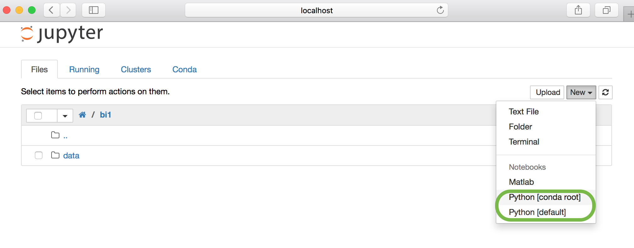
To start a new Python notebook, click on the right-hand side of the application window and select New (the expanded menu is shown in the screen shot above). This will give you several options for new notebook kernels depending on what is installed on your computer. In the above screenshot, there are two available Python kernels and one Matlab kernel. When starting a notebook, you should choose Python 3 if it is available or conda(root) .

Once you start a new notebook, you will be brought to the following screen.

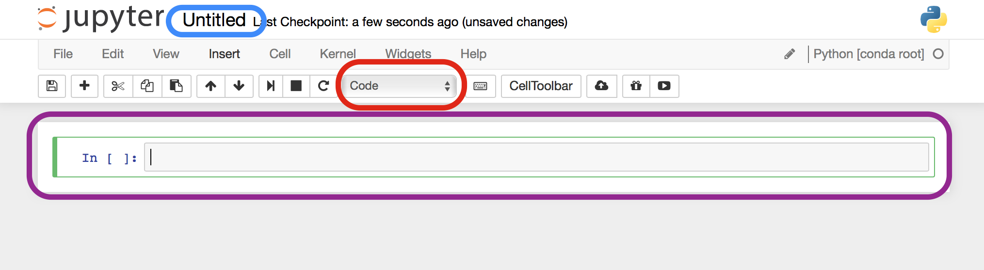
Welcome to your first look at a Jupyter notebook!

There are many available buttons for you to click. The three most important components of the notebook are highlighted in colored boxes.

• In blue is the name of the notebook. By clicking this, you can rename the notebook.
• In red is the cell formatting assignment. By default, it is registered as code, but it can also be set to markdown as described later.
• In purple, is the code cell. In this cell, you can type an execute Python code as well as text that will be formatted in a nicely readable format.

Selecting a Kernel

A kernel is a server that enables you to run commands within Jupyter Notebook. It is visible via a prompt window that logs all your actions in the notebook, making it helpful to refer to when encountering errors. You'll be prompted to select a kernel when you open a new notebook, however, if you are opening an existing notebook you will want to ensure that you are using the correct kernel. The commands for selecting and changing kernels are in the Kernel menu.

When you select or switch a kernel, you may want to use the navigate to Kernel in the menu, select Restart/ClearOutlook. The Restart/ClearOutlook option ensures that the correct kernel will operate.

You can always check what version of Python you are running by typing the following into a code cell.

 # Check what version of Python.  Should be 3.5. 
 import sys
 sys.version

Writing & running code

The following information is adapted from Griffin Chure's

All code you write in the notebook will be in the code cell. You can write single lines, to entire loops, to complete functions. As an example, we can write and evaluate a print statement in a code cell, as is shown below.

If you would like to write several lines of code, hit Enter to continue entering code into another line. To execute the code, we can simply hit Shift + Enter while our cursor is in the code cell.

 # This is a comment and is not read by Python
 print('Hello! This is the print function. Python will print this line below')

 Hello! This is the print function. Python will print this line below

We can also write a 'for' loop as an example of executing multiple lines of code at once.

 # Write a basic for loop. In this case a range of numbers 0-4.
 for i in range(5):
# Multiply the value of i by two and assign it to a variable. 
temp_variable = 2 * i

# Print the value of the temp variable.
print(temp_variable)

 0
 2
 4
 6
 8

There are two other useful keyboard shortcuts for running code:

• Alt + Enter runs the current cell and inserts a new one below
• Ctrl + Enter run the current cell and enters command mode.

For more keyboard shortcuts, check out weidadeyue's .

If you would like more details on running code in Jupyter Notebooks, please go through the following short tutorial by by contributors to the Jupyter project. This tutorial touches on start and stopping the kernel and using multiple kernels (e.g., Python and R) in one notebook.

Writing Text

The following information is adapted from Griffin Chure's

Arguably the most useful component of the Jupyter Notebook is the ability to interweave code and explanatory text into a single, coherent document. Through out the Data Institute (and one's everyday workflow), we encourage all code and plots should be accompanied with explanatory text.

Each cell in a notebook can exist either as a code cell or as a text-formatting cell called a markdown cell. Markdown is a mark-up language that very easily converts to other type-setting formats such as HTML and PDF.

Whenever you make a new cell, its default assignment will be a code cell. This means when you want to write text, you will need to specifically change it to a markdown cell. You can do this by clicking on the drop-down menu that reads code' (highlighted in red in the second figure of this page) and selecting 'Markdown'. You can then type in the code cell and all Python syntax highlighting will be removed.

Resources for Learning Markdown

• Review the NEON tutorial Git 04: Markdown Files
• Adam Pritchard's

Saving & Quitting

The following information is adapted from Griffin Chure's

Jupyter notebooks are set up to autosave your work every 15 or so minutes. However, you should not rely on the autosave feature! Save your work frequently by clicking on the floppy disk icon located in the upper left-hand corner of the toolbar.

To navigate back to the root of your Jupyter notebook server, you can click on the Jupyter logo at any time.

To quit your Jupyter notebook, you can simply close the browser window and the Jupyter notebook server running in your terminal.

Converting to HTML and PDF

In addition to sharing notebooks in the.ipynb format, it may useful to convert these notebooks to highly-portable formats such as HTML and PDF.

To convert, you can either use the dropdown menu option

File -> download as -> ...

or via the command line by using the following lines:

 jupyter nbconvert --to pdf notebook_name.ipynb 

Where "notebook_name.ipynb" matches the name of the notebook you want to convert. Prior to converting the notebook, you must be in the same working directory as your notebook or use the correct file path from your current working directory.

Converting to PDF requires both Pandoc and LaTeX to be installed. You can find out more in the .

If you prefer to convert to a different format, like HTML, you simply change the file type. jupyter nbconvert --to html notebook_name.ipynb Read more on what formats you can convert to and more about the .

Additional Resources

Using Jupyter Notebooks

• Jupyter Documentation on
• Griffin Chure's multi-part course on . Much of the material above is adapted from .
• Jupyter Project's

Using Python

• Software Carpentry's
• Data Carpentry's
• Many, many others that a simple web search will bring up...