AGÕæÈË°Ù¼ÒÀÖ¹Ù·½ÍøÕ¾

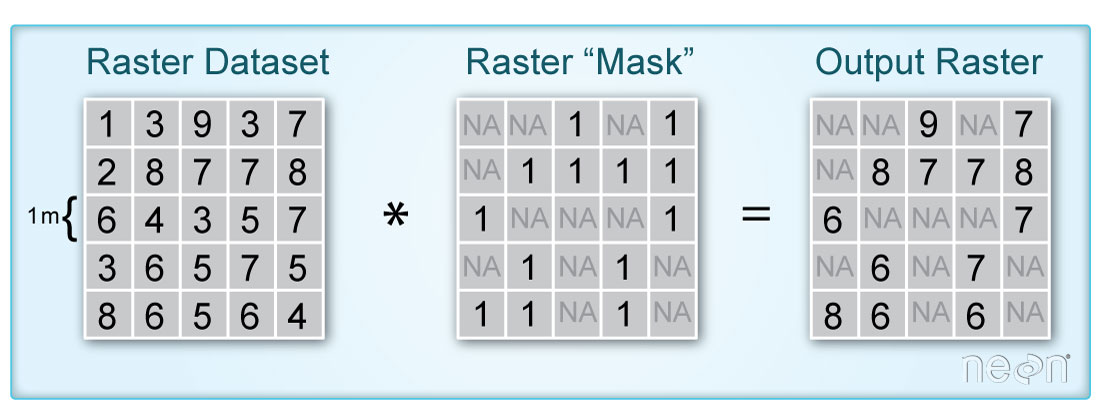
In this tutorial, we demonstrate how to remove parts of a raster based on pixel values using a mask we create. A mask raster layer contains pixel values of either 1 or 0 to where 1 represents pixels that will be used in the analysis and 0 are pixels that are assigned a value of nan (not a number). This can be useful in a number of scenarios, when you are interested in only a certain portion of the data, or need to remove poor-quality data, for example.

import os
import copy
import numpy as np
import numpy.ma as ma
import rasterio as rio
from rasterio.plot import show, show_hist
import requests
import zipfile
import matplotlib.pyplot as plt
from matplotlib import colors
import matplotlib.patches as mpatches
%matplotlib inline

Read in the datasets

Download Lidar Elevation Models and Vegetation Indices from TEAK

To start, we will download the NEON Lidar Aspect and Spectrometer Vegetation Indices (including the NDVI) which are provided in geotiff (.tif) format. Use the download_url function below to download the data directly from the cloud storage location.

# function to download data stored on the internet in a public url to a local file
def download_url(url,download_dir):
    if not os.path.isdir(download_dir):
        os.makedirs(download_dir)
    filename = url.split('/')[-1]
    r = requests.get(url, allow_redirects=True)
    file_object = open(os.path.join(download_dir,filename),'wb')
    file_object.write(r.content)

# define the urls for downloading the Aspect and NDVI geotiff tiles
aspect_url = "https://storage.googleapis.com/neon-aop-products/2021/FullSite/D17/2021_TEAK_5/L3/DiscreteLidar/AspectGtif/NEON_D17_TEAK_DP3_320000_4092000_aspect.tif"
ndvi_url = "https://storage.googleapis.com/neon-aop-products/2021/FullSite/D17/2021_TEAK_5/L3/Spectrometer/VegIndices/NEON_D17_TEAK_DP3_320000_4092000_VegetationIndices.zip"

# download the raster data using the download_url function
download_url(aspect_url,'.\data')
download_url(ndvi_url,'.\data')

# display the contents in the ./data folder to confirm the download completed
os.listdir('./data')

We can use zipfile to unzip the VegetationIndices folder in order to read the NDVI file (which is included in the zipped folder).

with zipfile.ZipFile("./data/NEON_D17_TEAK_DP3_320000_4092000_VegetationIndices.zip","r") as zip_ref:
    zip_ref.extractall("./data")

os.listdir('./data')

Now that the files are downloaded, we can read them in using rasterio.

aspect_file = os.path.join("./data",'NEON_D17_TEAK_DP3_320000_4092000_aspect.tif')
aspect_dataset = rio.open(aspect_file)
aspect_data = aspect_dataset.read(1)

# preview the aspect data
aspect_data

Define and view the spatial extent so we can use this for plotting later on.

ext = [aspect_dataset.bounds.left,
       aspect_dataset.bounds.right,
       aspect_dataset.bounds.bottom,
       aspect_dataset.bounds.top]
ext

Plot the aspect map and histogram.

fig, (ax1, ax2) = plt.subplots(1, 2, figsize=(14,6))
aspect_map = show(aspect_dataset, ax=ax1);
im = aspect_map.get_images()[0]
fig.colorbar(im, label = 'Aspect (degrees)', ax=ax1) # add a colorbar
ax1.ticklabel_format(useOffset=False, style='plain') # turn off scientific notation

show_hist(aspect_dataset, bins=50, histtype='stepfilled',
          lw=0.0, stacked=False, alpha=0.3, ax=ax2);
ax2.set_xlabel("Canopy Height (meters)");
ax2.get_legend().remove()

plt.show();

Classify aspect by direction (North and South)

aspect_reclass = aspect_data.copy()

# classify North and South as 1 & 2
aspect_reclass[np.where(((aspect_data>=0) & (aspect_data<=45)) | (aspect_data>=315))] = 1 #North - Class 1
aspect_reclass[np.where((aspect_data>=135) & (aspect_data<=225))] = 2 #South - Class 2
# West and East are unclassified (nan)
aspect_reclass[np.where(((aspect_data>45) & (aspect_data<135)) | ((aspect_data>225) & (aspect_data<315)))] = np.nan 

Read in the NDVI data to a rasterio dataset.

ndvi_file = os.path.join("./data",'NEON_D17_TEAK_DP3_320000_4092000_NDVI.tif')
ndvi_dataset = rio.open(ndvi_file)
ndvi_data = ndvi_dataset.read(1)

Plot the NDVI map and histogram.

fig, (ax1, ax2) = plt.subplots(1, 2, figsize=(14,6))
ndvi_map = show(ndvi_dataset, cmap = 'RdYlGn', ax=ax1);
im = ndvi_map.get_images()[0]
fig.colorbar(im, label = 'NDVI', ax=ax1) # add a colorbar
ax1.ticklabel_format(useOffset=False, style='plain') # turn off scientific notation

show_hist(ndvi_dataset, bins=50, histtype='stepfilled',
          lw=0.0, stacked=False, alpha=0.3, ax=ax2);
ax2.set_xlabel("NDVI");
ax2.get_legend().remove()

plt.show();

Plot the classified aspect map to highlight the north and south facing slopes.

# Plot classified aspect (N-S) array
fig, ax = plt.subplots(1, 1, figsize=(6,6))
cmap_NS = colors.ListedColormap(['blue','white','red'])
plt.imshow(aspect_reclass,extent=ext,cmap=cmap_NS)
plt.title('TEAK North & South Facing Slopes')
ax=plt.gca(); ax.ticklabel_format(useOffset=False, style='plain') #do not use scientific notation 
rotatexlabels = plt.setp(ax.get_xticklabels(),rotation=90) #rotate x tick labels 90 degrees

# Create custom legend to label N & S
white_box = mpatches.Patch(facecolor='white',label='East, West, or NaN')
blue_box = mpatches.Patch(facecolor='blue', label='North')
red_box = mpatches.Patch(facecolor='red', label='South')
ax.legend(handles=[white_box,blue_box,red_box],handlelength=0.7,bbox_to_anchor=(1.05, 0.45), 
          loc='lower left', borderaxespad=0.);

Mask Data by Aspect and NDVI

Now that we have imported and converted the classified aspect and NDVI rasters to arrays, we can use information from these to find create a new raster consisting of pixels are North facing and have an NDVI > 0.4.

#Mask out pixels that are north facing:
# first make a copy of the ndvi array so we can further select a subset
ndvi_gtpt4 = ndvi_data.copy()
ndvi_gtpt4[ndvi_data<0.4]=np.nan

fig, ax = plt.subplots(1, 1, figsize=(6,6))
plt.imshow(ndvi_gtpt4,extent=ext)
plt.colorbar(); plt.set_cmap('RdYlGn'); 
plt.title('TEAK NDVI > 0.4')
ax=plt.gca(); ax.ticklabel_format(useOffset=False, style='plain') #do not use scientific notation 
rotatexlabels = plt.setp(ax.get_xticklabels(),rotation=90) #rotate x tick labels 90 degrees

#Now include additional requirement that slope is North-facing (i.e. aspectNS_array = 1)
ndvi_gtpt4_north = ndvi_gtpt4.copy()
ndvi_gtpt4_north[aspect_reclass != 1] = np.nan

fig, ax = plt.subplots(1, 1, figsize=(6,6))
plt.imshow(ndvi_gtpt4_north,extent=ext)
plt.colorbar(); plt.set_cmap('RdYlGn'); 
plt.title('TEAK, North Facing & NDVI > 0.4')
ax=plt.gca(); ax.ticklabel_format(useOffset=False, style='plain') #do not use scientific notation 
rotatexlabels = plt.setp(ax.get_xticklabels(),rotation=90) #rotate x tick labels 90 degrees

It looks like there aren't that many parts of the North facing slopes where the NDVI > 0.4. Can you think of why this might be? Hint: consider both ecological reasons and how the flight acquisition might affect NDVI.

Let's also look at where NDVI > 0.4 on south facing slopes.

#Now include additional requirement that slope is Sorth-facing (i.e. aspect_reclass = 2)
ndvi_gtpt4_south = ndvi_gtpt4.copy()
ndvi_gtpt4_south[aspect_reclass != 2] = np.nan

fig, ax = plt.subplots(1, 1, figsize=(6,6))
plt.imshow(ndvi_gtpt4_south,extent=ext)
plt.colorbar(); plt.set_cmap('RdYlGn'); 
plt.title('TEAK, South Facing & NDVI > 0.4')
ax=plt.gca(); ax.ticklabel_format(useOffset=False, style='plain') #do not use scientific notation 
rotatexlabels = plt.setp(ax.get_xticklabels(),rotation=90) #rotate x tick labels 90 degrees

Export Masked Raster to Geotiff

We can also use rasterio to write out the geotiff file. In this case, we will just copy over the metadata from the NDVI raster so that the projection information and everything else is correct. You could create your own metadata dictionary and change the coordinate system, etc. if you chose, but we will keep it simple for this example.

out_meta = ndvi_dataset.meta.copy()
with rio.open('TEAK_NDVIgtpt4_South.tif', 'w', **out_meta) as dst:
    dst.write(ndvi_gtpt4_south, 1)

For peace of mind, let's read back in this raster that we generated and confirm that the contents are identical to the array that we used to generate it. We can do this visually, by plotting it, and also with an equality test.

out_file = "TEAK_NDVIgtpt4_South.tif"
new_dataset = rio.open(out_file)
show(new_dataset);

# use np.array_equal to check that the contents of the file we read back in is the same as the original array 
np.array_equal(new_dataset.read(1),ndvi_gtpt4_south,equal_nan=True)