Tutorial
Forecast Beetle Richness and Abundance and Submit Forecasts to the NEON Ecological Forecast Challenge
Last Updated: Apr 4, 2025
AG真人百家乐官方网站 this tutorial
Learning objectives
- Overview of the theme for the
- How to create a simple forecast for the Beetle Communities theme
- How to submit/score a forecast to evaluate its accuracy
- How to use the NEON Forecast Challenge resources in your research and teaching
Target user groups for this tutorial
This tutorial is intended to be used by ecological forecasters at any stage of expertise and may be used as a learning tool as an introduction to forecasting properties of ecological populations or communities. Below, we provide code for introductory examples to walk through the entire process of creating and submitting a forecast to the NEON Ecological Forecasting challenge. This includes:
- Accessing target datasets of NEON ground beetle richness and abundance
- Accessing weather forecast data to use as drivers in models predicting beetle data
- How to use the
fablepackage for R to specify and fit models - How to submit a forecast to the forecast challenge
Upon completing this tutorial, participants should be able to create and submit forecasts to the Beetle Communities theme of the EFI RCN NEON Ecological Forecasting challenge.
Things you will need to complete this tutorial
You will need a current version of R (v4.2 or newer) to complete this tutorial. We also recommend the RStudio IDE to work with R.
To complete the workshop the following packages will need to be installed:
R Packages to Install
Prior to starting the tutorial ensure that the following packages are installed.
-
tidyverse:
install.packages("tidyverse")(collection of R packages for data manipulation, analysis, and visualisation) -
lubridate:
install.packages("lubridate")(working with dates and times) -
tsibble:
install.packages("tsibble")(working with timeseries data) -
fable:
install.packages("fable")(running forecasts) -
fabletools:
install.packages("fabletools")(helper functions for using fable) -
remotes:
install.packages("remotes")(accessing packages from github) -
neon4cast:
remotes::install_github('eco4cast/neon4cast')(package from NEON4cast challenge organizers to assist with forecast building and submission) -
score4cast:
remotes::install_github('eco4cast/score4cast')(package to score forecasts)
The following code chunk should be run to install packages.
install.packages('tidyverse')

install.packages('lubridate')

install.packages('tsibble')

install.packages('fable')

install.packages('fabletools')

install.packages('remotes')

remotes::install_github('eco4cast/neon4cast')

remotes::install_github("eco4cast/score4cast")
Then load the packages.
version$version.string

## [1] "R version 4.4.3 (2025-02-28)"

library(tidyverse)

library(lubridate)

library(tsibble)

library(fable)

library(fabletools)

library(neon4cast)

library(score4cast)
Introduction
The Challenge has been organized by the Ecological Forecasting Initiative Research Coordination Network ().
The Challenge asks the scientific community to produce ecological forecasts of future observations of ecological data that will be collected and published by the National Ecological Observatory Network (NEON). The Challenge is split into that span aquatic and terrestrial systems, and population, community, and ecosystem processes across a broad range of ecoregions. We are excited to use this Challenge to learn more about the predictability of ecological processes by forecasting NEON data before it is collected.
Which modeling frameworks, mechanistic processes, and statistical approaches best capture community, population, and ecosystem dynamics? These questions are answerable by a community generating a diverse array of forecasts. The Challenge is open to any individual or team from anywhere around the world that wants to submit forecasts. Learn more about how you can participate
Goals for forecasts of ecological communities
Ecologists are interested in tracking changes in the number of individual organisms over time (count data of abundance). Numbers of each species will change due to births, deaths, and movement in (immigration) or out (emigration) of populations. The abundance of an ecological community is the sum of the number of individuals of each species. For example, in a hypothetical community of beetles sampled in Year 1 (time=1) , Species A has 10 individuals, Species B has 40 individuals and Species C has 50 individuals, giving a community abundance of 100. In subsequent years the abundance may increase, decrease or remain constant. A forecast may use this sequence of observations over time to predict how many individuals will occur in the next year (time=2), or a number of years into the future (time n). How far into the future we predict is known as the forecast horizon. The accuracy of the prediction is then compared to new observations and a new prediction is made.
Ecologists are also interested in tracking changes in the number of species over time (Species richness over time without species identity) and in species turnover over time steps where the identity of the species is known. In the example above there are three species (A,B,C) but over time this can change if for example Species C was to decline from 10 to zero individuals then the species richness would be 2, or increase if two previously unobserved species (D & E) arrive into the community, the species richness would be 4. Note that the loss of species A and the arrival of D and E gives a net species richness of 4, but without keeping track of the identity of the species we may be unaware of how community composition is changing over time.
Ecological communities change for many reasons and so it is important to understand the drivers of changes in abundance or species richness by adding abiotic variables into the models. By knowing how species change over time we can use the driving variables to predict, or forecast, the values for the abundance and species richness variables for the ecological communities into the future.
Overview of the theme
What: Forecast abundance and/or richness of ground beetles (carabids) collected in pitfall traps, standardized to sampling effort (trap night). More information about the NEON data product (DP1.10022.001, Ground beetles sampled from pitfall traps) we are forecasting can be found . Note that we are not downloading the target dataset from the NEON data portal. Rather, we will download a version of the dataset that has been simplified and preformatted for this challenge by the EFI RCN. An example script to preformat the target data from the EFI RCN can be found . Specifically, the targets are:
-
abundance: Total number of carabid individuals per trap-night, estimated each week of the year at each NEON site -
richness: Total number of unique 鈥榮pecies鈥� in a sampling bout for each NEON site each week.
Where: All 47 terrestrial NEON sites.
You can download metadata for all NEON sites as follows:
# To download the NEON site information table:

neon_site_info <- read_csv("/sites/default/files/NEON_Field_Site_Metadata_20231026.csv")
This table has information about the field sites, including location, ecoregion, and other useful metadata (e.g. elevation, mean annual precipitation, temperature, and NLCD class).
Or, you can load a more targeted list of just the sites included in the Beetle Communities theme:
site_data <- read_csv("https://raw.githubusercontent.com/eco4cast/neon4cast-targets/main/NEON_Field_Site_Metadata_20220412.csv") %>%

  dplyr::filter(beetles == 1)
For this tutorial, we are going to focus on the NEON site at Ordway-Swisher Biological Station (OSBS), which is located in Domain 03 (D03) in Florida.
If you're interested to learn more about downloading and exploring NEON data beyond beetles at OSBS, follow this link to get an overview of NEON's data products, how to download the data, and how to interact visualize and analyze the data.
When: Target data are available as early as 2013 at some sites, and data are available at all sites from 2019 on. Pitfall trap deployments are typically two weeks in duration (i.e., a sampling bout lasts two weeks), and traps are collected and redeployed throughout the growing season at each NEON site. Note that the target data for The Challenge are standardized to represent beetle abundance per trap night. Because pitfall trap samples need to be sorted and individuals counted and identified, the latency for data publication can be nearly a year. In this tutorial we will train our models on data from 2013-2021 and we will make forecasts for the 2022 season so that we can score them immediately.
Check current ground beetle data availability on the .
Determining a reference date (the first day of the forecast) and a forecast horizon (the time window that is being forecast) are two major challenges when forecasting population and community data. Other themes in the NEON Ecological Forecast Challenge focus on targets that are derived from instrument data, e.g., dissolved Oxygen or temperature in lakes, that are collected at a high frequency (e.g., > 1 Hz) and available in near-real-time (e.g., latency < 1 day). In practice, forecasts for these types of data have horizons that are typically a week to a month because they use output from weather forecasts (e.g., NOAA GEFS forecasts) as drivers in their models. These forecasts can be evaluated and updated as new data roll in, and new weather forecasts are published. This approach is known as "iterative near-term ecological forecasting" ().
In contrast, population and community data are often available at a much lower frequency (e.g., bi-weekly or annual sampling bouts) with a much higher latency (e.g., 6 months to a year) because of the effort that is required to collect and process samples and publish the data. Thus, the goals and applications will likely be different for forecasts of these types of data. There is still an opportunity to iterate, and update forecasts, but over a much longer time period. For more information on NEON's Provisional and Released data refer to this link here.
QUESTION: What are some use-cases for forecasts of ecological populations and communities that you are interested in pursuing?
Forecasting NEON beetle communities
Define spatial and temporal parameters for our forecast
Here we set some values for variables in our code to identify the NEON site we will be working with and the forecast start and end dates. This will allow us to easily adapt this code for future runs at different sites and forecasting different time windows.
Choose a NEON site:
# choose site

my_site = "OSBS"
Choose forecast start and end dates:
# date where we will start making predictions

forecast_startdate <- "2022-01-01" #fit up through 2021, forecast 2022 data


# date where we will stop making predictions

forecast_enddate <- "2025-01-01"
Note that the forecast_startdate will be renamed reference_datetime when we submit our forecast to the The Challenge. As the parameter name indicates, this date represents the beginning of the forecast. For this tutorial, we are using a forecast_startdate, or reference_datetime, that is in the past so that we can evaluate the accuracy of our forecasts at the end of this tutorial.
The forecast_enddate is used to determine the forecast horizon. In this example, we are setting a horizon to extend into the future.
If you want to create a true forecast to submit to the challenge, you will want to set your forecast_startdate as today's date. However, you will likely need to wait until next year before you can evaluate your forecast performance because you will need to wait for the data to be collected, processed, and published.
Read in the data
We begin by first looking at the historic data - called the 'targets'. These data are available with a latency of approximately 330 days. Here is how you read in the data from the targets file available from the EFI server.
# beetle targets are here

url <- "https://sdsc.osn.xsede.org/bio230014-bucket01/challenges/targets/project_id=neon4cast/duration=P1W/beetles-targets.csv.gz"


# read in the table

targets <- read_csv(url) %>%
  mutate(datetime = as_date(datetime)) %>%  # set proper formatting
  dplyr::filter(site_id == my_site,  # filter to desired site
                datetime < "2022-12-31") # excluding provisional data
Visualise the target data
Let's take a look at the targets data!
targets[100:110,]

## # A tibble: 11 脳 6
##    project_id site_id datetime duration variable observation
##    <chr>      <chr>   <date>   <chr>    <chr>          <dbl>
##  1 <NA>       <NA>    NA       <NA>     <NA>              NA
##  2 <NA>       <NA>    NA       <NA>     <NA>              NA
##  3 <NA>       <NA>    NA       <NA>     <NA>              NA
##  4 <NA>       <NA>    NA       <NA>     <NA>              NA
##  5 <NA>       <NA>    NA       <NA>     <NA>              NA
##  6 <NA>       <NA>    NA       <NA>     <NA>              NA
##  7 <NA>       <NA>    NA       <NA>     <NA>              NA
##  8 <NA>       <NA>    NA       <NA>     <NA>              NA
##  9 <NA>       <NA>    NA       <NA>     <NA>              NA
## 10 <NA>       <NA>    NA       <NA>     <NA>              NA
## 11 <NA>       <NA>    NA       <NA>     <NA>              NA
It is good practice to examine the dataset before proceeding with analysis:
targets %>%
  as_tsibble(index = datetime, key = variable) %>%
  autoplot() +
  facet_grid(variable ~ ., scales = "free_y") +
  theme_bw() +
  theme(legend.position = "none")
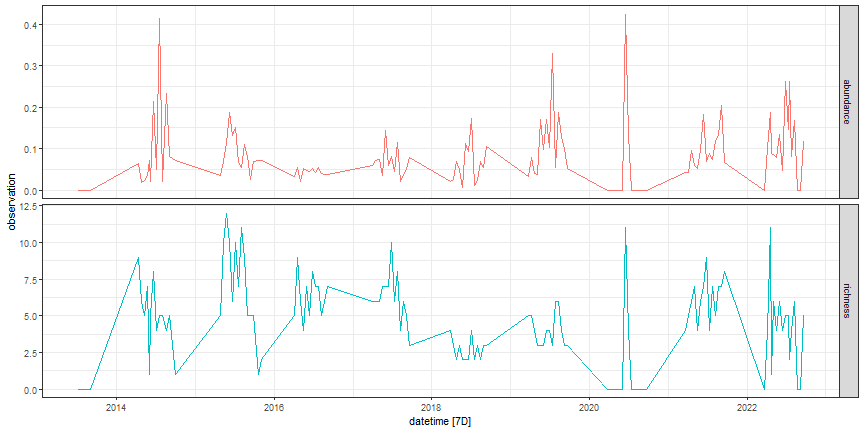
Figure: Beetle targets data at OSBS
Create the training dataset
We will train our forecast models on target data from the beginning of the dataset until our forecast_startdate, which we set above.
targets_train <- targets %>%
  filter(datetime < forecast_startdate) %>%
  pivot_wider(names_from = variable, values_from = observation) %>%
  as_tsibble(index = datetime)
Example forecasts: some simple models
In this tutorial, we will begin by producing two "null model" forecasts using functions available in the fable package for R. The MEAN null model will forecast abundance based on the historical mean and standard deviation in the training data. The NAIVE null model is a random walk model that generates a forecast based on the current observation plus process uncertainty. We will then use the TSLM function to create simple linear regression models to predict beetle abundances using daily temperature (mean daily temperature at 2m height) and precipitation (daily cumulative precipitation) estimates produced from CMIP6 model runs from 1950-2050. While these data do not represent actual observations of temperature and precipitation at the NEON site, they have been fit to historical data, so past dates in the simulated data should capture general trends at the site and values for future dates should represent a realistic forecast of meteorological variables into the future.
An overview of the models we will fit to the data in this tutorial:
- Null models
-
fable::MEAN(): Historical mean and standard deviation -
fable::NAIVE(): Random walk model assuming future data are current data plus process uncertainty
-
- Regression models with meteorology drivers (accessed from )
- Temperature: Daily mean temperature from CMIP6 model runs
- Precipitation: Daily cumulative precipitation from CMIP6 model runs
- Temperature + Precipitation
Here, we use CMIP6 data drivers as both training and forecasting data for simplicity and the ability to generate forecasts further into the future compared to other target data with shorter data latencies.
At the end of this tutorial, we will compare the performance of our best regression model against the two null models.
Forecast beetle abundance: null models
Here, we fit our two null models to the training data and then create forecasts for 2022-2024. Note that we are using a log(x + 1) transform (using the log1p() function) for the abundance data in all of our models. This is a common transform for abundance data for communities, which are typically log-normal, but with zeros. We are keeping the model simple for this example, but you could substitute generalized linear regression models, zero-inflated models, or other approaches better model the distribution of beetle abundances.
# specify and fit models

# Using a log(x + 1) transform on the abundance data

mod_fits <- targets_train %>%
  tsibble::fill_gaps() %>% # gap fill the data for the random walk model
  fabletools::model(
    mod_mean = fable::MEAN(log1p(abundance)), # generate a forecast from the historical mean plus the standard deviation of the historical data
    mod_naive = fable::NAIVE(log1p(abundance))) # random walk model, requires gap filling. Generates a forecast from the current observation plus random process noise


# make a forecast

fc_null <- mod_fits %>%
  fabletools::forecast(h = "3 years")
Next, we can visualize our two null model forecasts.
# visualize the forecast

fc_null %>%
  autoplot(targets_train) +
  facet_grid(.model ~ ., scales = "free_y") +
  theme_bw()
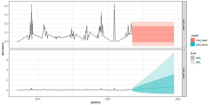
Figure: NULL forecasts of ground beetle abundance at OSBS
Note the difference in the scale of the y-axis between the two forecasts. How might this affect your use of the two different models as null models?
Forecast beetle abundance: regression models
Regression on meteorological model outputs allows us to make predictions about future field seasons based on CMIP6 projections. We downloaded model outputs from using the RopenMeto package, which you can install using: remotes::install_github("FLARE-forecast/RopenMeteo"). More information about the simulations that produced the drivers used in this example can be found .
So we do not overwhelm the open-meteo API, we have made the data used in this tutorial available as a .
The data we're using in this example were generated by the CMCC_CM2_VHR4 meteorological model.
Other predictor variables beyond meteorology data are appropriate for forecasting. Just remember that the driver data for forecasting are an out-of-sample observation (also forecasted) such that it can be used to generate a prediction of beetle richness and abundance. That is why NEON's meteorological data from OSBS are not used to generate beetle forecasts, as we can only observe up to the current time that the forecast starts. Additionally, the hand-off from directly observed meteorological data to forecasted data introduces additional uncertainty to forecasts that we have currently omitted. For the sake of simplicity, we have trained the data on past CMIP6 model projections that have been corrected to the nearest observations and then forecasted with CMIP6's CMCC_CM2_VHR4 model projection ensembles.
# Get meteorology data

path_to_clim_data <- "https://data.cyverse.org/dav-anon/iplant/projects/NEON/ESA2024/forecasting_beetles_workshop/modeled_climate_2012-2050_OSBS_CMCC_CM2_VHR4.csv"


clim_long <- read_csv(path_to_clim_data)  %>%
        filter(datetime <= forecast_enddate)


# make a tsibble object

clim_long_ts <- clim_long %>%
  as_tsibble(index = datetime,
             key = c(variable, model_id))


# make wide

clim_wide <- clim_long %>%
  select(-unit) %>%
  pivot_wider(names_from = variable, values_from = prediction)
Let's take a look at the data. The dotted line indicates our forecast_startdate.
# visualize meteorology data

clim_long_ts %>%
  ggplot(aes(datetime, prediction)) +
  geom_line() +
  facet_grid(variable ~ ., scales = "free_y") +
  geom_vline(xintercept = lubridate::as_date(forecast_startdate),
             lty = 2) +
  theme_bw() +
  theme(legend.position = "none")
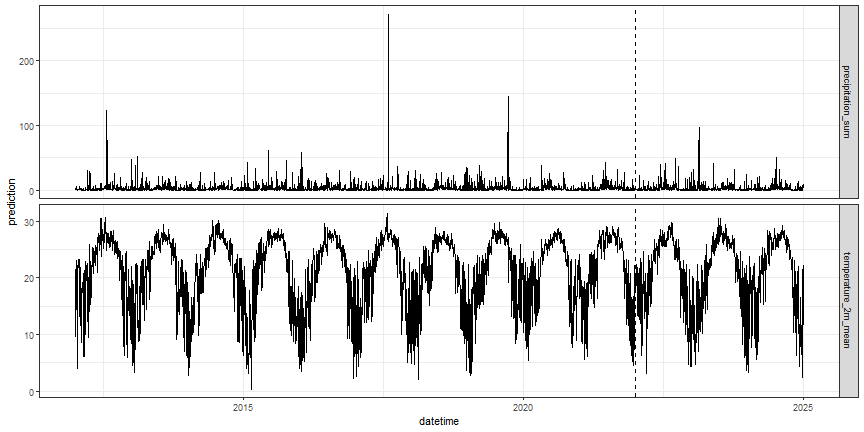
Figure: modeled meteorology data at OSBS
Next, we will break up the meteorology data into a training set (clim_past) and a dataset to use for forecasting (clim_future).
# subset into past and future datasets, based on forecast_startdate

clim_past <- clim_wide %>%
  filter(datetime < forecast_startdate,
         datetime > "2012-01-01")


clim_future <- clim_wide %>%
  filter(datetime >= forecast_startdate,
         datetime <= forecast_enddate)
Now, combine target and meteorology data to make a training dataset.
# combine target and meteorology data into a training dataset

targets_clim_train <- targets_train %>%
  left_join(clim_past)
Next, specify and fit simple linear regression models using fable::TSLM(), and examine the model fit statistics.
# specify and fit model

mod_fit_candidates <- targets_clim_train %>%
  fabletools::model(
    mod_temp = fable::TSLM(log1p(abundance) ~ temperature_2m_mean),
    mod_precip = fable::TSLM(log1p(abundance) ~ precipitation_sum),
    mod_temp_precip = fable::TSLM(log1p(abundance) ~ temperature_2m_mean + precipitation_sum))


# look at fit stats and identify the best model using AIC, where the lowest AIC is the best model

fabletools::report(mod_fit_candidates) %>%
  select(`.model`, AIC)

## # A tibble: 3 脳 2
##   .model            AIC
##   <chr>           <dbl>
## 1 mod_temp        -129.
## 2 mod_precip      -128.
## 3 mod_temp_precip -127.
Now, plot the predicted versus observed abundance data.
# visualize model fit

# augment reformats model output into a tsibble for easier plotting

fabletools::augment(mod_fit_candidates) %>%
  ggplot(aes(x = datetime)) +
  geom_line(aes(y = abundance, lty = "Obs"), color = "dark gray") +
  geom_line(aes(y = .fitted, color = .model, lty = "Model")) +
  facet_grid(.model ~ .) +
  theme_bw()
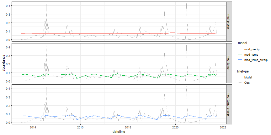
Figure: TSLM predictions of beetle abundances at OSBS compared against observed data
We could use all of these models to make an ensemble forecast, but for simplicity, we will just take the best model (lowest AICc), and use that to create a forecast:
# focus on temperature model for now

mod_best_lm <- mod_fit_candidates %>% select(mod_temp)

report(mod_best_lm)

## Series: abundance
## Model: TSLM
## Transformation: log1p(abundance)
##
## Residuals:
##       Min        1Q    Median        3Q       Max
## -0.088452 -0.038339 -0.015457 -0.002563  0.281881
##
## Coefficients:
##                      Estimate Std. Error t value Pr(>|t|)
## (Intercept)         -0.128599   0.198481  -0.648    0.523
## temperature_2m_mean  0.007980   0.007614   1.048    0.305
##
## Residual standard error: 0.08527 on 25 degrees of freedom
## Multiple R-squared: 0.04208,	Adjusted R-squared: 0.003768
## F-statistic: 1.098 on 1 and 25 DF, p-value: 0.30466

# make a forecast

# filter "future" meteorology data to target model

fc_best_lm <- mod_best_lm %>%
  fabletools::forecast(
    new_data =
      clim_future %>%
      as_tsibble(index = datetime))
Visualize the forecast.
# visualize the forecast

fc_best_lm %>%
  autoplot(targets_train) +
  facet_grid(.model ~ .) +
  theme_bw()
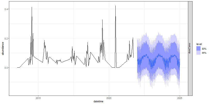
Figure: TSLM forecast of beelte abundance at OSBS
Does this forecast seem reasonable?
How to submit a forecast to the NEON Forecast Challenge
Detailed guidelines on how to submit a forecast to the NEON Forecast Challenge can be found . The requires the following columns:
-
project_id: use "neon4cast" -
model_id: the short name of the model defined as the model_id in your registration. The model_id should have no spaces. model_id should reflect a method to forecast one or a set of target variables and must be unique to the neon4cast challenge. -
datetime: forecast timestamp. Format%Y-%m-%d %H:%M:%Swith UTC as the time zone. Forecasts submitted with a%Y-%m-%dformat will be converted to a full datetime assuming UTC mid-night. -
reference_datetime: The start of the forecast; this should be 0 times steps in the future. There should only be one value ofreference_datetimein the file. Format is%Y-%m-%d %H:%M:%Swith UTC as the time zone. Forecasts submitted with a%Y-%m-%dformat will be converted to a full datetime assuming UTC mid-night. -
duration: the time-step of the forecast. Use the value ofP1Dfor a daily forecast,P1Wfor a weekly forecast, andPT30Mfor 30 minute forecast. This value should match the duration of the target variable that you are forecasting. Formatted as -
site_id: code for NEON site. -
family: name of the probability distribution that is described by the parameter values in the parameter column (see list below for accepted distribution). An ensemble forecast as a family of ensemble. See note below about family -
parameter: the parameters for the distribution (see note below about the parameter column) or the number of the ensemble members. For example, the parameters for a normal distribution are calledmuandsigma. -
variable: standardized variable name. It must match the variable name in the target file. -
prediction: forecasted value for the parameter in the parameter column
To submit our example forecast, we can take the output from the fabletools::forecast() function we used above and feed it into neon4cast::efi_format() to format the output for submissions to The Challenge. We also need to add a few additional columns.
# update dataframe of model output for submission

fc_best_lm_efi <- fc_best_lm %>%
  mutate(site_id = my_site) %>% #efi needs a NEON site ID
  neon4cast::efi_format() %>%
  mutate(
    project_id = "neon4cast",
    model_id = "bet_abund_example_tslm_temp",
    reference_datetime = forecast_startdate,
    duration = "P1W")
What does the content of the submission look like?
head(fc_best_lm_efi)

## # A tibble: 6 脳 10
##   datetime   site_id parameter model_id     family variable prediction project_id reference_datetime duration
##   <date>     <chr>   <chr>     <chr>        <chr>  <chr>         <dbl> <chr>      <chr>              <chr>
## 1 2022-01-01 OSBS    1         bet_abund_e鈥� ensem鈥� abundan鈥�    -0.0629 neon4cast  2022-01-01         P1W
## 2 2022-01-01 OSBS    2         bet_abund_e鈥� ensem鈥� abundan鈥�     0.134  neon4cast  2022-01-01         P1W
## 3 2022-01-01 OSBS    3         bet_abund_e鈥� ensem鈥� abundan鈥�    -0.122  neon4cast  2022-01-01         P1W
## 4 2022-01-01 OSBS    4         bet_abund_e鈥� ensem鈥� abundan鈥�    -0.0430 neon4cast  2022-01-01         P1W
## 5 2022-01-01 OSBS    5         bet_abund_e鈥� ensem鈥� abundan鈥�     0.0954 neon4cast  2022-01-01         P1W
## 6 2022-01-01 OSBS    6         bet_abund_e鈥� ensem鈥� abundan鈥�    -0.0189 neon4cast  2022-01-01         P1W


# visualize the EFI-formatted submission

fc_best_lm_efi %>%
  as_tsibble(index = datetime,
             key = c(model_id, parameter)) %>%
  ggplot(aes(datetime, prediction, color = parameter)) +
  geom_line() +
  facet_grid(model_id ~ .) +
  theme_bw()
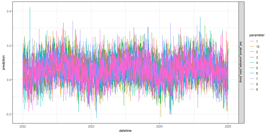
Figure: TSLM forecast submission file for OSBS, parameter indicates emsemble member
Lastly, if you feel so inclined, you can submit your forecast outputs file as an entry to The Challenge to be scored. If you want to submit a file, you will (1) need to and (2) you cannot have the word "example" in your filename or model_id. In the example below, we are including the "example" text string in the file and model names so it is not evaluated as part of the challenge.
# file name format is: theme_name-year-month-day-model_id.csv


# set the theme name

theme_name <- "beetles"


# set your submission date

file_date <- Sys.Date()


# make sure the model_id in the filename matches the model_id in the data

# NOTE: having the text string "example" in the file name will prevent this

# submission from being displayed on the challenge dashboard or being included

# in statistics about challenge participation.

efi_model_id <- "bet_abund_example_tslm_temp"


# format the file name

forecast_file <- paste0(theme_name,"-",file_date,"-",efi_model_id,".csv.gz")


# write the file to your working directory

write_csv(fc_best_lm_efi, forecast_file)


# submit the file

neon4cast::submit(forecast_file = forecast_file)
Evaluating your forecast
How your submission will be scored
The Challenge implements methods from the scoringRules R package to calculate the Continuous Rank Probability Score (CRPS) via the score4cast package, where a lower CRPS score indicates higher forecast accuracy. CRPS uses information about the variance of the forecasts as well as the estimated mean to calculate the score by comparing it with the observation. There is some balance between accuracy and precision. The forecasts will also be compared with 'null' models (RW and climatology). More information can be found in the or the score4cast package from EFI organizers .
You can view past submissions to the Beetle Communities theme .
You can also download the raw scores from the bucket directly, for example:
# This example requires the `arrow` package

# install.packages("arrow")

library(arrow)


# what is your model_id?

# my_mod_id <- "bet_abund_example_tslm_temp"

# my_mod_id <- "bet_example_mod_null"

my_mod_id <- "bet_example_mod_naive"


# format the URL

my_url <- paste0(

  "s3://anonymous@bio230014-bucket01/challenges/scores/parquet/project_id=neon4cast/duration=P1W/variable=abundance/model_id=",

  my_mod_id,

  "?endpoint_override=sdsc.osn.xsede.org")


# bind dataset

ds_mod_results <- arrow::open_dataset(my_url)


# get recs for dates that are scored

my_scores <- ds_mod_results %>%

  filter(!is.na(crps)) %>%

  collect()


head(my_scores)
How to score your own forecast
For immediate feedback, we can use the targets data from 2022 to score our forecast for the 2022 field season at OSBS.
# filter to 2022 because that is the latest release year

# 2023 is provisional and most sites do not yet have data reported

targets_2022 <- targets %>%
  dplyr::filter(
    datetime >= "2022-01-01",
    datetime < "2023-01-01",
    variable == "abundance",
    observation > 0)


# list of target site dates for filtering mod predictions

target_site_dates_2022 <- targets_2022 %>%
  select(site_id, datetime) %>% distinct()


# filter model forecast data to dates where we have observations

mod_results_to_score_lm <- fc_best_lm_efi %>%
  left_join(target_site_dates_2022,.) %>%
  dplyr::filter(!is.na(parameter))


# score the forecasts

mod_scores <- score(
  forecast = mod_results_to_score_lm,
  target = targets_2022)


head(mod_scores)

## # A tibble: 4 脳 17
##   model_id      reference_datetime site_id datetime   family variable observation   crps   logs   mean median
##   <chr>         <chr>              <chr>   <date>     <chr>  <chr>          <dbl>  <dbl>  <dbl>  <dbl>  <dbl>
## 1 bet_abund_ex鈥� 2022-01-01         OSBS    2022-04-04 sample abundan鈥�      0.102  0.0345 -1.51  0.0347 0.0449
## 2 bet_abund_ex鈥� 2022-01-01         OSBS    2022-04-18 sample abundan鈥�      0.188  0.107  -0.487 0.0236 0.0307
## 3 bet_abund_ex鈥� 2022-01-01         OSBS    2022-04-25 sample abundan鈥�      0.0877 0.0190 -1.59  0.109  0.103
## 4 bet_abund_ex鈥� 2022-01-01         OSBS    2022-08-08 sample abundan鈥�      0.169  0.0465 -1.08  0.101  0.0870
## # 鈩� 6 more variables: sd <dbl>, quantile97.5 <dbl>, quantile02.5 <dbl>, quantile90 <dbl>, quantile10 <dbl>,
## #   horizon <drtn>
Are these scores better than our null models? Here, we will score the mod_mean and mod_naive models, and combine the null model scores with the scores for our best_lm forecast above. Then we can compare.
# get scores for the mean and naive models

# the fc_null object has scores from both models

# note: we need to add site_id back in for efi_format() to work

fc_null_efi <- fc_null %>%
  mutate(site_id = my_site) %>% #efi needs a NEON site ID
  neon4cast::efi_format()


# filter to dates where we have target data from 2022

mod_results_to_score_null <- fc_null_efi %>%
  left_join(target_site_dates_2022,.) %>%
  dplyr::filter(!is.na(parameter))


# score the forecasts for those dates

mod_null_scores <- score(
  forecast = mod_results_to_score_null,
  target = targets_2022)


# stack the scores for our best_lm and the null models

# forcing reference_datetime to be the same type in both tables

# so they will stack

all_mod_scores <- bind_rows(
  mod_null_scores %>% mutate(
    reference_datetime = as.character(reference_datetime)),
  mod_scores %>% mutate(
    reference_datetime = as.character(reference_datetime)))
Before we visualize the scores, we can visualize the target 2022 observations and compare them against the forecast ensembles (parameters) among all three models. Each individual line in the figure below represents a single forecast ensemble and all the lines together represents the forecast's uncertainty. The points represent the direct observed target data and assumes there is no uncertainty.
mod_results_to_score_lm <- mod_results_to_score_lm |> select(site_id,datetime,parameter,model_id,family,variable,prediction)


rbind(mod_results_to_score_null,mod_results_to_score_lm) %>%
  ggplot(., aes(datetime, prediction, color = model_id, group=interaction(parameter, model_id))) +
  geom_line(lwd = 1)+
  geom_point(aes(datetime, observation), color = "black", size = 6, inherit.aes = F, data = targets_2022)+
  ylab("Abundance")+
  theme_classic()
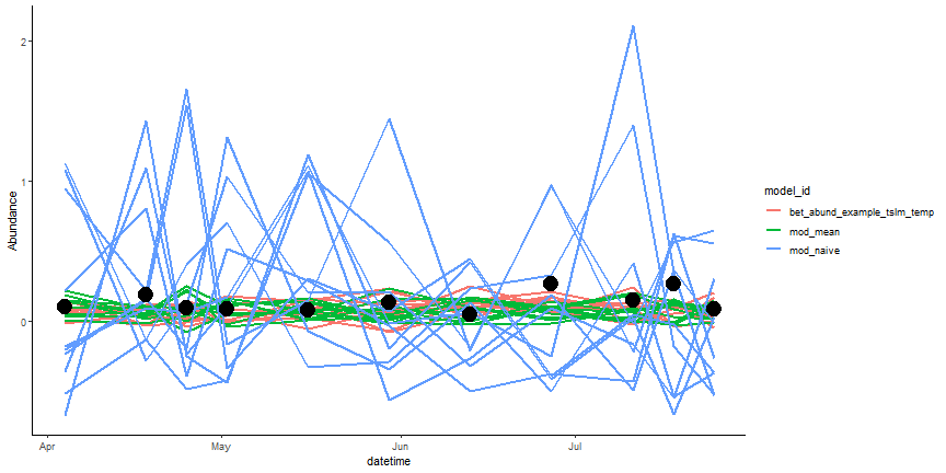
Figure: Compare Forecasts to Raw Data. Ensemble forecasts are the lines and the black circles are the direct observations.
Let's plot the scores. Remember, lower scores indicate better forecast accuracy.
all_mod_scores %>%
  ggplot(aes(datetime, crps, color = model_id)) +
  geom_line() +
  theme_bw() +
  ggtitle("Forecast scores over time at OSBS for 2022")

Figure: Forecast scores (CRPS) for models predicting beetle abundance at the OSBS NEON site during the 2022 field season
- Which model(s) did best?
- What might explain the differences in scores between the different models?
What's next?
- The forecasts we created here were relatively simple. What are ideas you have to improve the forecasts?
- How could you expand on this forecasting exercise? More sites? Different forecast horizons?
- How could you apply what you have learned here in your research or teaching?
Acknowledgements
This tutorial is based in part off of tutorials created by Freya Olsson for the and examples created by Carl Boettiger for the .