AGÕæÈË°Ù¼ÒÀÖ¹Ù·½ÍøÕ¾

The purpose of this tutorial is to introduce users to accessing NEON data for expanding metagenomic analyses. The tutorial is being run in conjunction with the workshop "FAIR Data and NEON Data discovery at the National Microbiome Data Collaborative", presented at the annual meeting of the Ecological Society of America. The purpose of this component is to provide a brief introduction to how to download NEON data, with a focus on those NEON data that can be used as metadata for the NMDC metagenomic analyses of NEON samples. We will provide some brief examples of how to download relevant NEON data for soil and aquatic samples, and then how to wrangle the data to link them to NEON metagenomic samples that have been run through the NMDC Edge pipeline.

install.packages("neonUtilities")

install.packages("neonOS")

install.packages("tidyverse")

The NEON Data Portal

NEON provides a wealth of data to assist with your research. is the best place to start looking for the data you want. There is a lot of information on this page. For now, we will have a quick tour.

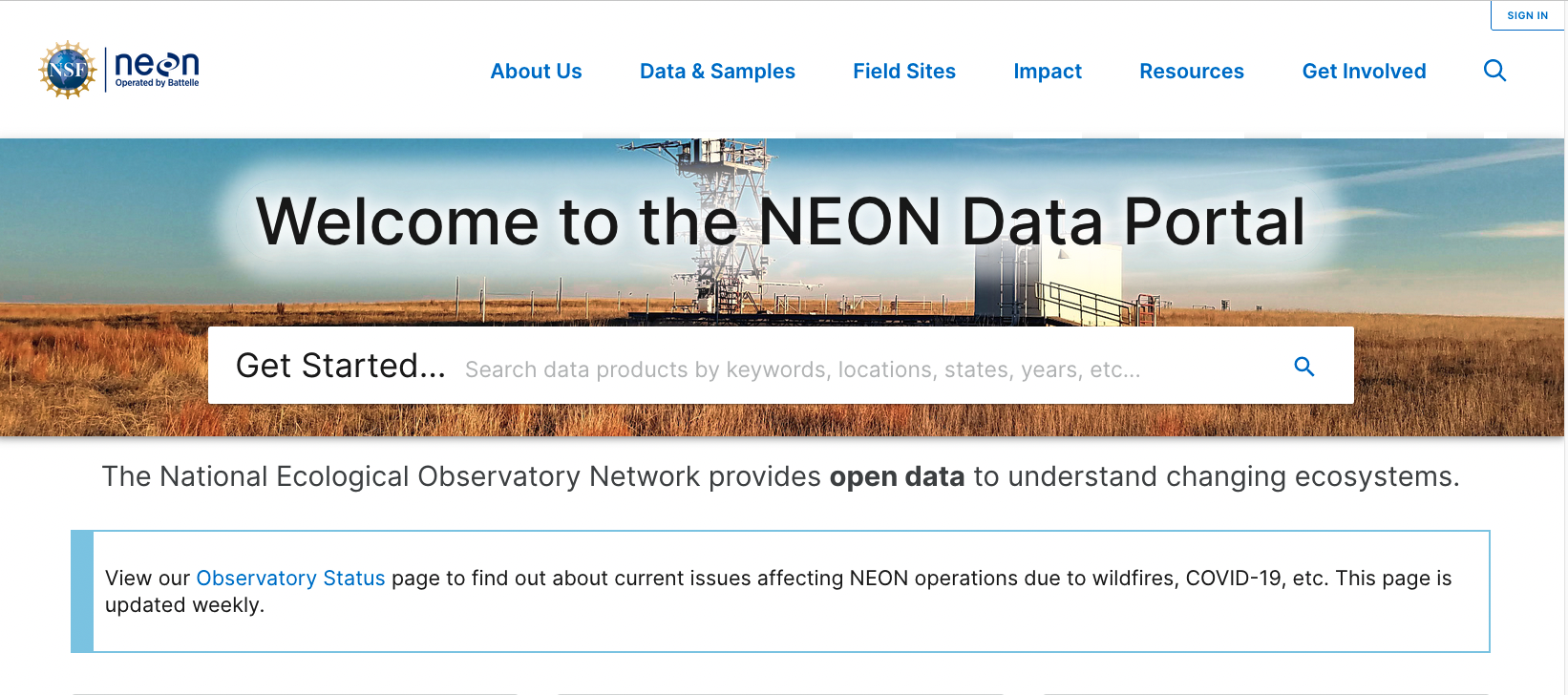
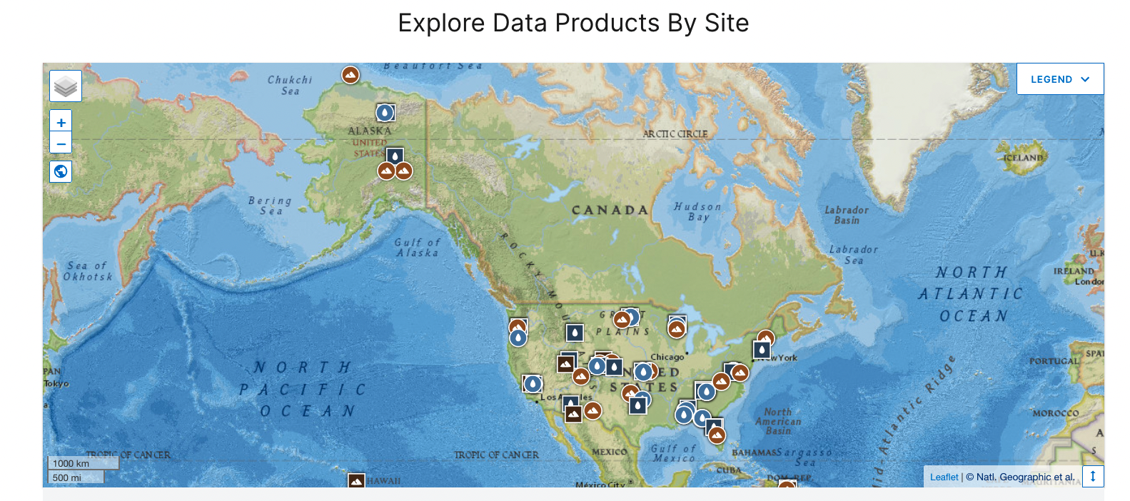
There are many ways to search the Data Portal, including searching by site. The page includes an interactive map.

Explore Data Products

From the Data Portal main page, Click on the EXPLORE button in the box called "Explore Data Products", or just , and you can search by key words or data product codes. For example, type 'metagenomics' in the Search field, and then scroll down through the results.

Click on the link to and the information for this data product will open in a new page. On this page there is a lot of useful information, including a description of the tables are included for the data, links to documents, a Quick Start guide, and much more. You of course are able to download data from this page, and can select specific sites and time ranges in an interactive table. However, in this tutorial we are going to use the neonUtilities R package to access the data.

NEON metadata for metagenomic data

Downloading data with neonUtilities

The metagenomics data available on the NEON website includes only the raw sequence files. The sample data available through the NMDC website have been processed through the NMDC Edge pipeline, and include taxonomic and functional genomic information. However, the NEON samples collected for metagenomic sequencing were also subjected to a wide range of measurements, including carbon and nitrogen isotopes, soil temperature, and pH. The following examples will help you to annontate the functional and taxonomic information of NEON samples on the NMDC data portal so they can be analyzed along with all other NEON data from the soil and aquatic samples.

We will start by accessing some soil chemical and physical measurements using the neonUtilities package. Though we will be using R to do this, it is still useful to look up the information on the NEON Data Portal. Go back to the , reset all filters, then type in "Soil physical and chemical properties" in the Search bar. Scroll down and click on "Soil physical and chemical properties, periodic" (DP1.10086.001).

With the information from the Data Portal, we can download this data product using the neonUtilities package. We will start with a subset of terrestrial sites. Go ahead and set up the following command in a text file in RStudio or text editor.

library(neonUtilities)



soilTrialSites = c("BONA","DEJU","HEAL","TOOL","BARR")



soilChem <- loadByProduct(

  dpID='DP1.10086.001',

  startdate = "2017-01",

  enddate = "2019-12",

  check.size = FALSE,

  site = soilTrialSites,

  package='expanded')

For full details on the loadByProduct() function, see the 'Use the neonUtilities Package' tutorial. Here we will just note some of the parameters. The dpID parameters is taken right from the Data Portal page for that data product. The startdate and enddate define the time range, and for the site parameter, we can enter a list of the four-letter codes for each site. The check.size we are leaving as FALSE, to prevent the function from warning us before big downloads. For example, if you do not specify a time range with startdate/enddate or define the sites to download using the site parameter, this will be a much bigger download and it is a good idea to leave this option at TRUE. If you are incorporating this code into a script as part of a pipeline, for example, then you should set this at FALSE.

Viewing the data

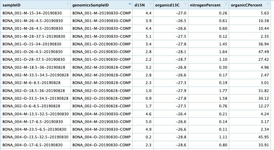
Once you have run this code and downloaded the data, we can have a look. The object returned by loadByProduct() function is a named list of data frames. To view or access each one, you can select them from the list of data frames using the $ operator. For example, if we would like to view the table sls_soilChemistry table in RStudio, then we can use the View() function:

View(soilChem$sls_soilChemistry)

You will then see a table open in a new tab in RStudio. You can see a lot of information in this table. This table contains multiple measurements of soil chemistry data that could be useful for metagenomics analysis. These include carbon and nitrogen isotopes (organic13C, d15N), percent C and N (organicCPercent, nitrogenPercent), and ratio of carbon to nitrogen (CNratio).

Take some time on your own to explore the other tables with this download.

Wrangling sample data for metagenomic samples

Now that you are familiar with downloading and viewing data through the neonUtilities package, we can start to focus on linking the data to the metagenomic samples. For soil samples, the DNA samples for metagenomics are combined from individual soil samples. This is why you will not see any of the chemistry data we just viewed corresponding to any metagenomic DNA sample directly. We need to access the list of samples that were combined to create a soil composite sample, so we can link these data directly. For this we look at the sls_metagenomicsPooling table.

View(soilChem$sls_metagenomicsPooling)

In this table the list for each composite DNA sample is in the column genomicsPooledIDList. For example, if we want to look at the list of samples used for the composite sample 'TOOL_043-O-20170719-COMP' (sample is in the genomicsSampleID field), we can pull up the list for the 11th sample in the table:

soilChem$sls_metagenomicsPooling$genomicsPooledIDList[11]

# you can check to confirm the first sample is TOOL_043-O-20170719-COMP

soilChem$sls_metagenomicsPooling[11,'genomicsSampleID']

The content of this field is a list demarcated by the pipe symbol ("|"):

"TOOL_043-O-5-7-20170719|TOOL_043-O-7.5-31-20170719|TOOL_043-O-32.5-27-20170719"

From the list you can see that there are three samples for the composite sample (there can be anywhere from 1-3 samples for each composite), all from plot TOOL_043 collected on 7/19/2017, and all from the organic soil horizon. Now we can observe the chemical measurements for those specific samples. We will use tidyverse to help get the fields from the table. Let's take the first one as an example:

library(tidyverse)



View(soilChem$sls_soilChemistry %>%

  filter(sampleID == "TOOL_043-O-5-7-20170719") %>%

  select(sampleID,d15N,organicd13C,CNratio))

We would like to be able to get these measurements for all the metagenomic subsamples. For this, we will first have to get the list for each composite sample and create a new table.

# split up the pooled list into new columns

genomicSamples <- soilChem$sls_metagenomicsPooling %>%

  tidyr::separate(genomicsPooledIDList, into=c("first","second","third"),sep="\\|",fill="right") %>%

  dplyr::select(genomicsSampleID,first,second,third)

# now view the table

View(genomicSamples)

Now we will adjust the table so that each sampleID is a row, with the genomicsSampleID listed for each sample:

genSampleExample <- genomicSamples %>% 

  tidyr::pivot_longer(cols=c("first","second","third"),values_to = "sampleID") %>%

  dplyr::select(sampleID,genomicsSampleID) %>%

  drop_na()

# now view

View(genSampleExample)

Now that you have all samples for each metagenomic sample listed, you can easily combine this table with other tables, using the sampleID. As an example we will go back to the soil chemistry data:

chemEx <- soilChem$sls_soilChemistry %>%

  dplyr::select(sampleID,d15N,organicd13C,nitrogenPercent,organicCPercent)



## now combine the tables 

combinedTab <- left_join(genSampleExample,chemEx, by = "sampleID") %>% drop_na()



View(combinedTab)

Merging metadata around composite samples

We now have a table that includes the genetic subsamples and their corresponding biogeochemical measurements. However, if we want to compare the biogeochemical data directly with the metagenomic genomic samples, you may want to merge the rows in the table back to a single row for each composite sample. This means we will need to average the chemical measurements across the subsamples for each composite sample. Care must be taken, however, when averaging across certain measurements (see in particular the example for averaging pH, below). Here is a basic example for our table:

genome_groups <- combinedTab %>%

  group_by(genomicsSampleID) %>%

  summarize_at(c("d15N","organicd13C","nitrogenPercent","organicCPercent"), mean)



View(genome_groups)

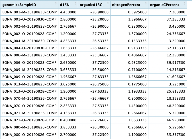
You now have a table that you can use to analyze your metagenomic data with some of the biogeochemical data. Hopefully the few examples on this page can help you get started. Please let us know if there is a particular type of data you are interested in analyzing with the metagenomic data and we will add to this page (or similar).

Additional examples for accessing data

Here are some other examples to help you get started with NEON metagenomic data

Merging pH measurements

The example above showing how to merge data works for many straightforward measurements, for which calculating the mean is logical. For pH measures, however, this won't work. Since pH is a logarithmic scale, averaging them will not work. Fortunately, the R package includes the function for averaging pH measurements. This function first converts each pH measure to hydrogen ion concentration [H+], averages the measures, then converts back to the logarithmic scale.

Below we show an example with the existing data. First we will create a new table with pH measurements, only keeping the samples from our metagenomic set:

soilpH_Example <- soilChem$sls_soilpH %>%

  dplyr::filter(sampleID %in% combinedTab$sampleID) %>%

  dplyr::select(sampleID,soilInWaterpH,soilInCaClpH)



# have a look at this table

View(soilpH_Example)

# now join with the existing table

combinedTab_pH <- left_join(combinedTab,soilpH_Example, by = "sampleID")

# and the final

View(combinedTab_pH)

Now, we can apply the same kind of tidyverse approach as the previous example, only using the mean_pH function:

library(respirometry)



genome_groups_pH <- combinedTab_pH %>%

  group_by(genomicsSampleID) %>%

  summarize_at(c("soilInWaterpH","soilInCaClpH"), mean_pH) 



View(genome_groups_pH)

One thing to note with the previous command is that all the other chemical data was lost when you ran the command. In this example we use two summarize_at commands to apply different functions to the two types of variables, and then left_join will combine them:

genome_groups_all <- combinedTab_pH %>%

  group_by(genomicsSampleID) %>%

  {left_join(

    summarize_at(.,vars("d15N","organicd13C","nitrogenPercent","organicCPercent"), mean),

    summarize_at(.,vars("soilInWaterpH","soilInCaClpH"), mean_pH)

  )}





View(genome_groups_all)

Downloading raw NEON metagenome data

If you are interested in accessing raw NEON metagenomic data (not processed as they are in NMDC) in order to run your own analyses, you can use the same neonUtilities package. The following code shows an example of how to download the raw sequence files.

library(neonUtilities)

library(dplyr)



#specify sites and/or date ranges depending on your research questions

metaGdata <- loadByProduct(dpID = 'DP1.10107.001',

                          startdate = "2018-01",

                          enddate = "2019-12",

                          check.size = FALSE,

                          package = 'expanded') 

The following code will produce a list all of the files in that data product loaded above.

rawFileInfo <- metaGdata$mms_rawDataFiles



urls_fordownload <- unique(rawFileInfo$rawDataFilePath)

If you want to only access a subset of those data, there are several options. One option is to use a list of known sample IDs. In the following example we subset around the list of samples from the earlier example in this tutorial. Note here that the dnaSampleID in the rawFileInfo table is different than the genomicsSampleId in the combinedTab table. The first step then is to create that field so we can select from it.

# Option a, create a list of samples from earlier example

targetsamples <- combinedTab$genomicsSampleID

# Create a genomicsSampleID from raw files table, and then subset this to samples

rawfiles_ids <- rawFileInfo %>%

  mutate(genomicsSampleID = gsub("-DNA[1,2,3]","",dnaSampleID)) %>%

  subset(genomicsSampleID %in% targetsamples) %>% 

  unique()



urls_fordownload <- unique(rawfiles_ids$rawDataFilePath)

Another option is to download the raw data in chunks:

# Option b

urls_fordownload <- unique(rawFileInfo$rawDataFilePath)[1:20] #for instance, the first 20 rows, and so on

Now write the urls to a text file

#put in whatever working directory you want

file_conn = file("./NEONmetagenome_downloadIDs.txt") 

writeLines(unlist(urls_fordownload), file_conn, sep="\n")

close(file_conn)

Now go into command line/terminal (you can use the Terminal tab in RStudio) and navigate to the directory where your text file is and run the following in the terminal:

wget -i NEONmetagenome_downloadIDs.txt

The gzipped fastq files will download to whichever directory you are in. this will work both locally and on an HPC.