AGÕæÈË°Ù¼ÒÀÖ¹Ù·½ÍøÕ¾

NEON observational data are diverse in both content and in data structure. Generally, data are published in a set of data tables, each of which corresponds to a particular activity: for example, several data products include a field collection data table, a sample processing data table, and a table of laboratory analytical results.

Joining data tables

Depending on the analysis you want to carry out, there may be data in multiple tables that you want to bring together. For example, it is very common that species identifications are in a different table from chemical composition or pathogen status. For species-specific analyses, you would need to draw on multiple tables. There are a variety of ways to do this, but one of the simplest is to join the tables and create a single flat table.

The Quick Start Guides and Data Product User Guides provide information about the relationships between different data tables, and we recommend you consult these documents for the data products you are working with to gain the full picture. Quick Start Guides (QSGs) are included in the download package when you download data via the Data Portal, and can also be viewed on the Data Product Details page for each data product; for example, see the page for . Scroll down to the Documentation section to see the QSG. The Data Product User Guide is also available in the Documentation menu.

To join related tables, the neonOS package provides the joinTableNEON() function, which checks the Table joining section of the QSG, and uses the information there to join the tables if possible. If the join isn't possible, or if it requires customized code, the function will return an informative error, and usually refer you to the QSG for more details.

Duplicates

One of the most common data entry errors that occurs in NEON OS data is duplicate entry. NEON data entry applications and ingest validation rules are designed to prevent duplicate entry where possible, but errors can't be avoided completely. Consequently, NEON metadata for each OS data product (the variables file) includes an indicator of which data fields, taken together, should define a unique record. This combination of fields is called the "primary key" for the data table. The neonOS function removeDups() uses these metadata to identify duplicate records. Depending on the content of the duplicate records, they may be resolved to a single record or marked as unresolvable - see below for details.

In this tutorial, we will de-duplicate and then join two data tables in the Aquatic plant bryophyte chemical properties (DP1.20063.001) data product, using it as an example to demonstrate the operation of these two functions. Then we will take a look at Mosquitoes sampled from CO2 traps (DP1.10043.001), which contains more complicated table relationships, and see how to modify the code to work with those tables.

Set Up R Environment and Download Data

First install and load the necessary packages.

# install packages. you can skip this step if 

# the packages are already installed

install.packages("neonUtilities")

install.packages("neonOS")

install.packages("ggplot2")



# load packages

library(neonUtilities)

library(neonOS)

library(ggplot2)

We'll use aquatic plant chemistry (DP1.20063.001) as the example dataset. Use the neonUtilities function loadByProduct() to download and read in the data. If you're not familiar with the neonUtilities package and how to use it to access NEON data, we recommend you follow the Download and Explore NEON Data tutorial before proceeding with this one.

Here, we'll use the same subset of aquatic plant chemistry data as in the Download and Explore tutorial. Get the data from the Prairie Lake, Suggs Lake, and Toolik Lake sites, specifying the 2022 data release.

apchem <- loadByProduct(dpID="DP1.20063.001", 
                        site=c("PRLA","SUGG","TOOK"), 
                        package="expanded",
                        release="RELEASE-2022",
                        check.size=F)

Copy each of the downloaded tables into the R environment.

list2env(apchem, .GlobalEnv)

Identify and Resolve Duplicates

As noted above, duplicate data entry is a common error in human data entry. removeDups() uses the definitional metadata in the variables file to identify duplicates. It requires two inputs: the data table, and the corresponding variables file.

apl_biomass <- removeDups(data=apl_biomass, 
                          variables=variables_20063)

## No duplicated key values found!

There were no duplicates found in the apl_biomass data table. A duplicateRecordQF quality flag has been added to the table, and you can confirm that there were no duplicates by checking the values of the flag.

unique(apl_biomass$duplicateRecordQF)

## [1] 0

All data have flag value = 0, indicating they are not duplicated. Let's check the apl_plantExternalLabDataPerSample table.

apl_plantExternalLabDataPerSample <- removeDups(
  data=apl_plantExternalLabDataPerSample, 
  variables=variables_20063)

10 duplicated key values found, representing 20 non-unique records. Attempting to resolve.
  |==========================================================================================| 100%
2 resolveable duplicates merged into matching records
2 resolved records flagged with duplicateRecordQF=1
16 unresolveable duplicates flagged with duplicateRecordQF=2

The function output tells you there were 20 duplicates (out of 26108 total data records). Four of those duplicates were resolved, leaving two records flagged as resolved duplicates, with duplicateRecordQF=1. The remaining 16 couldn't be resolved, and were flagged with duplicateRecordQF=2.

What does it mean for duplicates to be resolved? Some duplicates represent identical data that have been entered multiple times, whereas some duplicates have the same values in the primary key, but differ in data values. removeDups() has a fairly narrow set of criteria for resolving to a single record:

1. If one data record has empty fields that are populated in the other record, the non-empty values are retained.
2. If records are identical except for uid, remarks, and/or personnel (identifiedBy, recordedBy, etc) fields, unique values are concatenated within the non-matching fields, separated by | (pipes).

Records that can be merged to a single record by these criteria are flagged with duplicateRecordQF=1. Records with mis-matched data that can't be merged are retained as-is and flagged with duplicateRecordQF=2.

Note that even in fully identical duplicates, the uid field (universal identifier) will always be unique. Thus the uid field in merged records will always contain the pipe-delimited set of uids of the original records.

What does this look like in practice? Let's look at the two resolved duplicates:

apl_plantExternalLabDataPerSample[which(
  apl_plantExternalLabDataPerSample$duplicateRecordQF==1),]

##                                                                          uid domainID siteID
## 55 cca9850e-165d-4cb7-9872-eff490c79ffa|1f5a5389-c18c-4fbf-81d6-9cd45e65f48a      D03   SUGG
## 60 e6cab47f-427b-47a9-a281-cbfe7c101fc3|368e16bb-23d4-4596-b624-b338777bc9bc      D03   SUGG
##     namedLocation collectDate              sampleID sampleCondition
## 55 SUGG.AOS.reach  2016-02-22 SUGG.20160222.UTFO.Q5    condition ok
## 60 SUGG.AOS.reach  2016-02-22 SUGG.20160222.UTFO.Q5    condition ok
##                                      laboratoryName analysisDate   analyzedBy sampleType replicate
## 55 Academy of Natural Sciences of Drexel University   2016-07-12 OKgcKejxXbI=         CN         1
## 60 Academy of Natural Sciences of Drexel University   2016-07-12 OKgcKejxXbI=         CN         1
##    sampleVolumeFiltered filterSize percentFilterAnalyzed  analyte analyteConcentration plantAlgaeLabUnits
## 55                   NA         25                   100   carbon                34.01            percent
## 60                   NA         25                   100 nitrogen                 2.84            percent
##    method externalRemarks  publicationDate      release duplicateRecordQF
## 55   <NA>            <NA> 20211221T225348Z RELEASE-2022                 1
## 60   <NA>            <NA> 20211221T225348Z RELEASE-2022                 1

You can see that both records have two pipe-delimited uids, and are flagged.

Let's look at the unresolveable duplicates:

apl_plantExternalLabDataPerSample[which(
  apl_plantExternalLabDataPerSample$duplicateRecordQF==2),]

##                                     uid domainID siteID  namedLocation collectDate              sampleID
## 1  5fa69a8b-d19e-40f1-84a8-e46ed08cdc59      D03   SUGG SUGG.AOS.reach  2014-07-09 SUGG.20140709.LISP2.1
## 2  cebefd95-f4c7-4e60-9b79-93efd3f27691      D03   SUGG SUGG.AOS.reach  2014-07-09 SUGG.20140709.LISP2.3
## 3  a4b6d931-b093-419e-bb69-0b684219405e      D03   SUGG SUGG.AOS.reach  2014-07-09 SUGG.20140709.LISP2.1
## 4  f462390b-2d4a-4aec-92e1-b46a740ec40d      D03   SUGG SUGG.AOS.reach  2014-07-09  SUGG.20140709.NULU.7
## 5  d4fa7f65-6b2b-46fa-9bca-529745970c56      D03   SUGG SUGG.AOS.reach  2014-07-09  SUGG.20140709.NULU.7
## 6  ab43c466-b235-4f3d-9146-a1f81a91012d      D03   SUGG SUGG.AOS.reach  2014-07-09 SUGG.20140709.LISP2.3
## 7  1140a4c2-139e-40dc-a14d-c2446e3a5664      D03   SUGG SUGG.AOS.reach  2014-07-09  SUGG.20140709.NULU.9
## 8  5201dc04-da3d-4bc2-b2bf-668ad4a3ddb5      D03   SUGG SUGG.AOS.reach  2014-07-09  SUGG.20140709.NULU.7
## 9  1e36cdeb-4e94-431d-8342-5ce5ff6ac6ae      D03   SUGG SUGG.AOS.reach  2014-07-09  SUGG.20140709.NULU.9
## 10 b98069a4-74fb-40d8-8b98-7a5aedea7912      D03   SUGG SUGG.AOS.reach  2014-07-09  SUGG.20140709.NULU.9
## 11 9633d367-bd10-4588-a6e2-cbe954327bf6      D03   SUGG SUGG.AOS.reach  2014-07-09  SUGG.20140709.NULU.9
## 12 309ccbe3-d4a8-4bd3-b773-85aa98dd7627      D03   SUGG SUGG.AOS.reach  2014-07-09 SUGG.20140709.LISP2.1
## 13 6d6b1da2-049f-439c-81c9-add482f6fab8      D03   SUGG SUGG.AOS.reach  2014-07-09 SUGG.20140709.LISP2.1
## 14 841e51f4-dcc9-45fc-937b-871678ff16f2      D03   SUGG SUGG.AOS.reach  2014-07-09 SUGG.20140709.LISP2.3
## 15 3e04c3a1-7e2f-4349-a1c2-822d736fc2cf      D03   SUGG SUGG.AOS.reach  2014-07-09  SUGG.20140709.NULU.7
## 16 431a4418-fdd0-4566-8791-d16ecfce76eb      D03   SUGG SUGG.AOS.reach  2014-07-09 SUGG.20140709.LISP2.3
##    sampleCondition                                   laboratoryName analysisDate   analyzedBy sampleType
## 1     condition ok Academy of Natural Sciences of Drexel University   2015-02-05 OKgcKejxXbI=         CN
## 2     condition ok Academy of Natural Sciences of Drexel University   2015-02-05 OKgcKejxXbI=         CN
## 3     condition ok Academy of Natural Sciences of Drexel University   2015-02-05 OKgcKejxXbI=         CN
## 4     condition ok Academy of Natural Sciences of Drexel University   2015-02-05 OKgcKejxXbI=         CN
## 5     condition ok Academy of Natural Sciences of Drexel University   2015-02-05 OKgcKejxXbI=         CN
## 6     condition ok Academy of Natural Sciences of Drexel University   2015-02-05 OKgcKejxXbI=         CN
## 7     condition ok Academy of Natural Sciences of Drexel University   2015-02-05 OKgcKejxXbI=         CN
## 8     condition ok Academy of Natural Sciences of Drexel University   2015-02-05 OKgcKejxXbI=         CN
## 9     condition ok Academy of Natural Sciences of Drexel University   2015-02-05 OKgcKejxXbI=         CN
## 10    condition ok Academy of Natural Sciences of Drexel University   2015-02-05 OKgcKejxXbI=         CN
## 11    condition ok Academy of Natural Sciences of Drexel University   2015-02-05 OKgcKejxXbI=         CN
## 12    condition ok Academy of Natural Sciences of Drexel University   2015-02-05 OKgcKejxXbI=         CN
## 13    condition ok Academy of Natural Sciences of Drexel University   2015-02-05 OKgcKejxXbI=         CN
## 14    condition ok Academy of Natural Sciences of Drexel University   2015-02-05 OKgcKejxXbI=         CN
## 15    condition ok Academy of Natural Sciences of Drexel University   2015-02-05 OKgcKejxXbI=         CN
## 16    condition ok Academy of Natural Sciences of Drexel University   2015-02-05 OKgcKejxXbI=         CN
##    replicate sampleVolumeFiltered filterSize percentFilterAnalyzed  analyte analyteConcentration
## 1          1                   NA         25                   100   carbon                38.22
## 2          1                   NA         25                   100 nitrogen                 2.26
## 3          1                   NA         25                   100 nitrogen                 1.98
## 4          1                   NA         25                   100   carbon                43.79
## 5          1                   NA         25                   100 nitrogen                 3.16
## 6          1                   NA         25                   100   carbon                39.77
## 7          1                   NA         25                   100   carbon                43.26
## 8          1                   NA         25                   100 nitrogen                 3.14
## 9          1                   NA         25                   100 nitrogen                 2.94
## 10         1                   NA         25                   100   carbon                43.20
## 11         1                   NA         25                   100 nitrogen                 3.00
## 12         1                   NA         25                   100   carbon                38.23
## 13         1                   NA         25                   100 nitrogen                 2.02
## 14         1                   NA         25                   100 nitrogen                 2.23
## 15         1                   NA         25                   100   carbon                43.93
## 16         1                   NA         25                   100   carbon                39.66
##    plantAlgaeLabUnits method   externalRemarks  publicationDate      release duplicateRecordQF
## 1             percent   <NA> Limnobium spongia 20220110T211020Z RELEASE-2022                 2
## 2             percent   <NA> Limnobium spongia 20220110T211020Z RELEASE-2022                 2
## 3             percent   <NA> Limnobium spongia 20220110T211020Z RELEASE-2022                 2
## 4             percent   <NA>     Nuphar Luteum 20220110T211020Z RELEASE-2022                 2
## 5             percent   <NA>     Nuphar Luteum 20220110T211020Z RELEASE-2022                 2
## 6             percent   <NA> Limnobium spongia 20220110T211020Z RELEASE-2022                 2
## 7             percent   <NA>     Nuphar Luteum 20220110T211020Z RELEASE-2022                 2
## 8             percent   <NA>     Nuphar Luteum 20220110T211020Z RELEASE-2022                 2
## 9             percent   <NA>     Nuphar Luteum 20220110T211020Z RELEASE-2022                 2
## 10            percent   <NA>     Nuphar Luteum 20220110T211020Z RELEASE-2022                 2
## 11            percent   <NA>     Nuphar Luteum 20220110T211020Z RELEASE-2022                 2
## 12            percent   <NA> Limnobium spongia 20220110T211020Z RELEASE-2022                 2
## 13            percent   <NA> Limnobium spongia 20220110T211020Z RELEASE-2022                 2
## 14            percent   <NA> Limnobium spongia 20220110T211020Z RELEASE-2022                 2
## 15            percent   <NA>     Nuphar Luteum 20220110T211020Z RELEASE-2022                 2
## 16            percent   <NA> Limnobium spongia 20220110T211020Z RELEASE-2022                 2

The key for this data table is the sample identifier and analyte, and here there are multiple records with the same sample identifier, both for carbon and nitrogen values. The most likely scenario is that these are unlabeled replicate analyses, i.e., the lab ran multiple analyses on the same samples for quality control purposes, but forgot to label them accordingly.

Now, how should you proceed with your analysis? Of course, that is up to you, and depends on your analysis. Because these appear to be unlabeled analytical replicates, I would probably average the analyte values, but a decision like this can't be made automatically - removeDups() can identify the records of concern, but what to do with them is a judgement call.

Of course, NEON scientists also review NEON data and identify duplicates as part of quality assurance and quality control procedures, and resolve them if possible. In the data download step above, we accessed RELEASE-2022. The data release is stable and reproducible over time, but duplicates you find in one release may be resolved in future releases.

Join Data Tables

If you are using neonOS to check for duplicates and also to join data tables, the duplicate step should always come first. Because duplicate identification uses the variables file to determine uniqueness of data records, the duplicate check step requires that the data match the variables file exactly, which they won't after being joined.

To join the apl_biomass and apl_plantExternalLabDataPerSample tables, we input both tables to the joinTableNEON() function. It uses the information provided in NEON quick start guides to determine whether the join is possible, and if it is, which fields to use to perform the join.

aqbc <- joinTableNEON(apl_biomass,
                      apl_plantExternalLabDataPerSample)

After joining tables, always take a look at the resulting table and make sure it makes sense. Errors in joining can easily result in completely nonsensical data. If you're not familiar with table joining operations, check out a lesson on the basics. The chapter on relational data in is a good one.

When checking your results, keep in mind that the default behavior of joinTableNEON() is a full join, i.e., all records from both original tables are retained, even if they don't match. For a small number of table pairs, the Quick Start Guide specifies a left join, and in those cases joinTableNEON() performs a left join.

Let's take a look at the aquatic plant table join:

nrow(apl_biomass)

## [1] 268

nrow(apl_plantExternalLabDataPerSample)

## [1] 572

nrow(aqbc)

## [1] 661

The number of rows in the joined table is larger than both of the original tables, but smaller than the sum of the original two. This suggests that most of the records in each of the original tables had a matching record in the other table, but some didn't.

View the full table:

View(aqbc)

(Table not displayed here due to size)

Here we can see we have several rows per chemSubsampleID for most chemSubsampleIDs. Each row corresponds to one of the chemical analytes, and the biomass data are repeated on each row. At the bottom of the table are a number of biomass records with no corresponding chemistry data; these explain why the merged table is larger than the original chemistry table.

This table structure is consistent with the original tables and with the intended join, so we're satisfied all is well. If you're working with a different data product and encounter something unexpected or undesirable in a joined table, contact NEON using the Contact Us page.

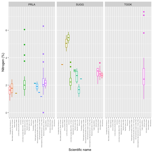
We can now connect chemical content to taxon, as in the Download and Explore NEON Data tutorial. Let's look at nitrogen content by species and site:

gg <- ggplot(subset(aqbc, analyte=="nitrogen"),
             aes(scientificName, analyteConcentration, 
                 group=scientificName, 
                 color=scientificName)) +
             geom_boxplot() + 
             facet_wrap(~siteID) +
        theme(axis.text.x=element_text(angle=90,
                                       hjust=1,
                                       size=4)) +
        theme(legend.position="none") +
        ylab("Nitrogen (%)") + 
        xlab("Scientific name")

gg

Other Input Options

After downloading the data above, we ran list2env() to make each table an independent object in the R environment, and then provided the tables to the two functions as-is. This worked because the names of the objects were identical to the table names, so the functions were able to figure out which tables they were. If the object names are not exactly equal to the table names, you will need to input the table names separately. If we hadn't used list2env(), this is how we would proceed:

bio.dup <- removeDups(data=apchem$apl_biomass,
                      variables=apchem$variables_20063,
                      table="apl_biomass")

chem.dup <- removeDups(data=apchem$apl_plantExternalLabDataPerSample,
                      variables=apchem$variables_20063,
                      table="apl_plantExternalLabDataPerSample")

aq.join <- joinTableNEON(table1=bio.dup, 
                         table2=chem.dup,
                         name1="apl_biomass",
                         name2="apl_plantExternalLabDataPerSample")

More Complicated Table Joins

In the aquatic plant chemistry example, we were able to join two tables in a single step. In some cases, the relationship between tables is more complicated, and joining is more difficult. In these cases, joinTableNEON() will provide an error message, and usually direct you to the Quick Start Guide for more information. Let's walk through how you can use this information, using Mosquitoes sampled from CO2 traps (DP1.10043.001) from Toolik Lake as an example.

mos <- loadByProduct(dpID="DP1.10043.001",
                     site="TOOL", 
                     release="RELEASE-2022",
                     check.size=F)

list2env(mos, .GlobalEnv)

Let's say we're interested in evaluating which mosquito species are found in which vegetation types. The species identifications are in the mos_expertTaxonomistIDProcessed table, and the trapping conditions are in the mos_trapping table. So we'll attempt to join those two tables.

mos.sp <- joinTableNEON(mos_trapping,

                        mos_expertTaxonomistIDProcessed)

Error in joinTableNEON(mos_trapping, mos_expertTaxonomistIDProcessed) : 
  Tables mos_trapping and mos_expertTaxonomistIDProcessed can't be joined directly, but can each be joined to a common table(s). Consult quick start guide for details.

The function returns an error, telling us it can't perform a simple join on the two tables, but there is a table they can each join to, which can be used to join them indirectly. As directed, we refer to the Quick Start Guide for DP1.10043.001, on the page.

From the QSG, we learn that mos_sorting is the intermediate table between mos_trapping and mos_expertTaxonomistIDProcessed.

First, let's join mos_trapping and mos_sorting:

mos.trap <- joinTableNEON(mos_trapping,
                          mos_sorting)

Now, this next step is a bit odd. We've created a merged table of mos_trapping and mos_sorting, but we know mos_expertTaxonomistIDProcessed can only join to mos_sorting. So we pass the merged table to joinTableNEON(), telling the function to use the join instructions for mos_sorting and mos_expertTaxonomistIDProcessed.

mos.tax <- joinTableNEON(mos.trap,
                         mos_expertTaxonomistIDProcessed,
                         name1="mos_sorting")

When you join data in this way, check carefully that the resulting table is structured logically and contains the data you expect it to. Looking at the merged table, we now have multiple records for each trapping event, with one record for each species captured in that event, plus a set of records for traps that either caught no mosquitoes or couldn't be deployed, and thus have no species identifications. This is consistent with the table join we performed, so everything appears to be correct.

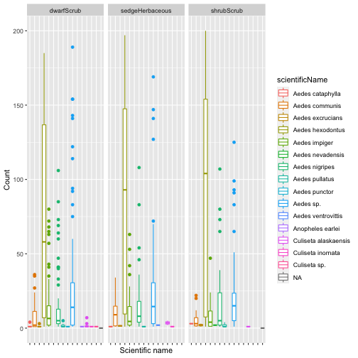
Let's take a look at species occurrence by habitat, as we set out to do:

gg <- ggplot(mos.tax, 
             aes(scientificName, individualCount, 
                 group=scientificName, 
                 color=scientificName)) +
             geom_boxplot() + 
        facet_wrap(~nlcdClass) +
        theme(axis.text.x=element_blank()) +
        ylab("Count") +
        xlab("Scientific name")

gg

## Warning: Removed 599 rows containing non-finite values (stat_boxplot).