Tutorial
Interacting with the PhenoCam Server using phenocamapi R Package
Last Updated: Apr 10, 2025
The is developed to simplify interacting with the dataset and perform data wrangling steps on PhenoCam sites' data and metadata.
This tutorial will show you the basic commands for accessing PhenoCam data through the PhenoCam API. The phenocampapi R package is developed and maintained by the PhenoCam team. The most recent release is available on GitHub (). can be found on how to merge external time-series (e.g. Flux data) with the PhenoCam time-series.
We begin with several useful skills and tools for extracting PhenoCam data directly from the server:
- Exploring the PhenoCam metadata
- Filtering the dataset by site attributes
- Downloading PhenoCam time-series data
- Extracting the list of midday images
- Downloading midday images for a given time range
Exploring PhenoCam metadata
Each PhenoCam site has specific metadata including but not limited to how a site is set up and where it is located, what vegetation type is visible from the camera, and its meteorological regime. Each PhenoCam may have zero to several Regions of Interest (ROIs) per vegetation type. The phenocamapi package is an interface to interact with the PhenoCam server to extract those data and process them in an R environment.
To explore the PhenoCam data, we'll use several packages for this tutorial.
library(data.table) #installs package that creates a data frame for visualizing data in row-column table format

library(phenocamapi)  #installs packages of time series and phenocam data from the Phenology Network. Loads required packages rjson, bitops and RCurl

library(lubridate)  #install time series data package

library(jpeg)
We can obtain an up-to-date data.frame of the metadata of the entire PhenoCam
network using the get_phenos() function. The returning value would be a
data.table in order to simplify further data exploration.
#Obtain phenocam metadata from the Phenology Network in form of a data.table

phenos <- get_phenos()


#Explore metadata table

head(phenos$site) #preview first six rows of the table. These are the first six phenocam sites in the Phenology Network

#> [1] "aafcottawacfiaf14e" "aafcottawacfiaf14n" "aafcottawacfiaf14w" "acadia"
#> [5] "admixpasture"       "adrycpasture"


colnames(phenos)  #view all column names.

#>  [1] "site"                      "lat"                       "lon"
#>  [4] "elev"                      "active"                    "utc_offset"
#>  [7] "date_first"                "date_last"                 "infrared"
#> [10] "contact1"                  "contact2"                  "site_description"
#> [13] "site_type"                 "group"                     "camera_description"
#> [16] "camera_orientation"        "flux_data"                 "flux_networks"
#> [19] "flux_sitenames"            "dominant_species"          "primary_veg_type"
#> [22] "secondary_veg_type"        "site_meteorology"          "MAT_site"
#> [25] "MAP_site"                  "MAT_daymet"                "MAP_daymet"
#> [28] "MAT_worldclim"             "MAP_worldclim"             "koeppen_geiger"
#> [31] "ecoregion"                 "landcover_igbp"            "dataset_version1"
#> [34] "site_acknowledgements"     "modified"                  "flux_networks_name"
#> [37] "flux_networks_url"         "flux_networks_description"

#This is all the metadata we have for the phenocams in the Phenology Network
Now we have a better idea of the types of metadata that are available for the Phenocams.
Remove null values
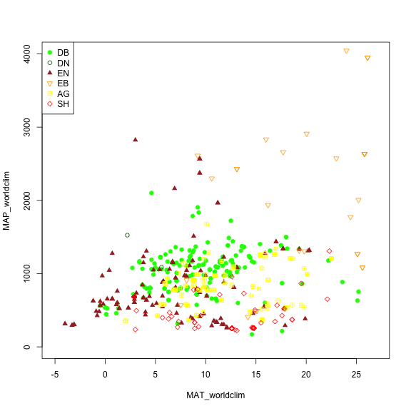
We may want to explore some of the patterns in the metadata before we jump into specific locations. Let's look at Mean Annual Precipitation (MAP) and Mean Annual Temperature (MAT) across the different field site and classify those by the primary vegetation type ('primary_veg_type') for each site.
| Abbreviation | Description | |----------|:-------------:|------:| | AG | agriculture | | DB | deciduous broadleaf | | DN | deciduous needleleaf | | EB | evergreen broadleaf | | EN | evergreen needleleaf | | GR | grassland | | MX | mixed vegetation (generally EN/DN, DB/EN, or DB/EB) | | SH | shrubs | | TN | tundra (includes sedges, lichens, mosses, etc.) | | WT | wetland | | NV | non-vegetated | | RF | reference panel | | XX | unspecified |
To do this we'd first want to remove the sites where there is not data and then plot the data.
# #Some sites do not have data on Mean Annual Precipitation (MAP) and Mean Annual Temperature (MAT).


# removing the sites with unknown MAT and MAP values

phenos <- phenos[!((MAT_worldclim == -9999)|(MAP_worldclim == -9999))]


# Making a plot showing all sites by their vegetation type (represented as different symbols and colors) plotting across meteorology (MAT and MAP) space. Refer to table to identify vegetation type acronyms.

phenos[primary_veg_type=='DB', plot(MAT_worldclim, MAP_worldclim, pch = 19, col = 'green', xlim = c(-5, 27), ylim = c(0, 4000))]

#> NULL

phenos[primary_veg_type=='DN', points(MAT_worldclim, MAP_worldclim, pch = 1, col = 'darkgreen')]

#> NULL

phenos[primary_veg_type=='EN', points(MAT_worldclim, MAP_worldclim, pch = 17, col = 'brown')]

#> NULL

phenos[primary_veg_type=='EB', points(MAT_worldclim, MAP_worldclim, pch = 25, col = 'orange')]

#> NULL

phenos[primary_veg_type=='AG', points(MAT_worldclim, MAP_worldclim, pch = 12, col = 'yellow')]

#> NULL

phenos[primary_veg_type=='SH', points(MAT_worldclim, MAP_worldclim, pch = 23, col = 'red')]

#> NULL


legend('topleft', legend = c('DB','DN', 'EN','EB','AG', 'SH'),
       pch = c(19, 1, 17, 25, 12, 23),
       col =  c('green', 'darkgreen', 'brown',  'orange',  'yellow',  'red' ))
Filtering using attributes
Alternatively, we may want to only include Phenocams with certain attributes in
our datasets. For example, we may be interested only in sites with a co-located
flux tower. For this, we'd want to filter for those with a flux tower using the
flux_sitenames attribute in the metadata.
# Create a data table only including the sites that have flux_data available and where the FLUX site name is specified

phenofluxsites <- phenos[flux_data==TRUE&!is.na(flux_sitenames)&flux_sitenames!='',
                         .(PhenoCam=site, Flux=flux_sitenames)] # return as table


#Specify to retain variables of Phenocam site and their flux tower name

phenofluxsites <- phenofluxsites[Flux!='']


# view the first few rows of the data table

head(phenofluxsites)

#>               PhenoCam                               Flux
#>                 <char>                             <char>
#> 1:        admixpasture                             NZ-ADw
#> 2: alercecosteroforest                             CL-ACF
#> 3:      alligatorriver                             US-NC4
#> 4:            amtsvenn                                 No
#> 5:    arkansaswhitaker                             US-RGW
#> 6:         arsbrooks10 US-Br1: Brooks Field Site 10- Ames
We could further identify which of those Phenocams with a flux tower and in
deciduous broadleaf forests (primary_veg_type=='DB').
#list deciduous broadleaf sites with a flux tower

DB.flux <- phenos[flux_data==TRUE&primary_veg_type=='DB',
                  site]  # return just the site names as a list


# see the first few rows

head(DB.flux)

#> [1] "alligatorriver" "bartlett"       "bartlettir"     "bbc1"           "bbc2"
#> [6] "bbc3"
PhenoCam time series
PhenoCam time series are extracted time series data obtained from regions of interest (ROI's) for a given site.
Obtain ROIs
To download the phenological time series from the PhenoCam, we need to know the
site name, vegetation type and ROI ID. This information can be obtained from each
specific PhenoCam page on the
or by using the get_rois() function.
# Obtaining the list of all the available regions of interest (ROI's) on the PhenoCam server and producing a data table

rois <- get_rois()


# view the data variables in the data table

colnames(rois)

#>  [1] "roi_name"          "site"              "lat"               "lon"
#>  [5] "roitype"           "active"            "show_link"         "show_data_link"
#>  [9] "sequence_number"   "description"       "first_date"        "last_date"
#> [13] "site_years"        "missing_data_pct"  "roi_page"          "roi_stats_file"
#> [17] "one_day_summary"   "three_day_summary" "data_release"


# view first few regions of of interest (ROI) locations

head(rois$roi_name)

#> [1] "aafcottawacfiaf14n_AG_1000"  "admixpasture_AG_1000"        "adrycpasture_AG_1000"
#> [4] "alercecosteroforest_EN_1000" "alligatorriver_DB_1000"      "almondifapa_AG_1000"
Download time series
The get_pheno_ts() function can download a time series and return the result
as a data.table.
Let's work with the
and specifically the ROI
we can run the following code.
# list ROIs for dukehw

rois[site=='dukehw',]

#>          roi_name   site      lat       lon roitype active show_link show_data_link
#>            <char> <char>    <num>     <num>  <char> <lgcl>    <lgcl>         <lgcl>
#> 1: dukehw_DB_1000 dukehw 35.97358 -79.10037      DB   TRUE      TRUE           TRUE
#>    sequence_number                                   description first_date  last_date site_years
#>              <num>                                        <char>     <char>     <char>     <char>
#> 1:            1000 canopy level DB forest at awesome Duke forest 2013-06-01 2024-12-30       10.7
#>    missing_data_pct                                            roi_page
#>              <char>                                              <char>
#> 1:              8.0 https://phenocam.nau.edu/webcam/roi/dukehw/DB_1000/
#>                                                                  roi_stats_file
#>                                                                          <char>
#> 1: https://phenocam.nau.edu/data/archive/dukehw/ROI/dukehw_DB_1000_roistats.csv
#>                                                             one_day_summary
#>                                                                      <char>
#> 1: https://phenocam.nau.edu/data/archive/dukehw/ROI/dukehw_DB_1000_1day.csv
#>                                                           three_day_summary data_release
#>                                                                      <char>       <lgcl>
#> 1: https://phenocam.nau.edu/data/archive/dukehw/ROI/dukehw_DB_1000_3day.csv           NA


# Obtain the decidous broadleaf, ROI ID 1000 data from the dukehw phenocam

dukehw_DB_1000 <- get_pheno_ts(site = 'dukehw', vegType = 'DB', roiID = 1000, type = '3day')


# Produces a list of the dukehw data variables

str(dukehw_DB_1000)

#> Classes 'data.table' and 'data.frame':	1414 obs. of  35 variables:
#>  $ date                : chr  "2013-06-01" "2013-06-04" "2013-06-07" "2013-06-10" ...
#>  $ year                : int  2013 2013 2013 2013 2013 2013 2013 2013 2013 2013 ...
#>  $ doy                 : int  152 155 158 161 164 167 170 173 176 179 ...
#>  $ image_count         : int  57 76 77 77 77 78 21 0 0 0 ...
#>  $ midday_filename     : chr  "dukehw_2013_06_01_120111.jpg" "dukehw_2013_06_04_120119.jpg" "dukehw_2013_06_07_120112.jpg" "dukehw_2013_06_10_120108.jpg" ...
#>  $ midday_r            : num  91.3 76.4 60.6 76.5 88.9 ...
#>  $ midday_g            : num  97.9 85 73.2 82.2 95.7 ...
#>  $ midday_b            : num  47.4 33.6 35.6 37.1 51.4 ...
#>  $ midday_gcc          : num  0.414 0.436 0.432 0.42 0.406 ...
#>  $ midday_rcc          : num  0.386 0.392 0.358 0.391 0.377 ...
#>  $ r_mean              : num  87.6 79.9 72.7 80.9 83.8 ...
#>  $ r_std               : num  5.9 6 9.5 8.23 5.89 ...
#>  $ g_mean              : num  92.1 86.9 84 88 89.7 ...
#>  $ g_std               : num  6.34 5.26 7.71 7.77 6.47 ...
#>  $ b_mean              : num  46.1 38 39.6 43.1 46.7 ...
#>  $ b_std               : num  4.48 3.42 5.29 4.73 4.01 ...
#>  $ gcc_mean            : num  0.408 0.425 0.429 0.415 0.407 ...
#>  $ gcc_std             : num  0.00859 0.0089 0.01318 0.01243 0.01072 ...
#>  $ gcc_50              : num  0.408 0.427 0.431 0.416 0.407 ...
#>  $ gcc_75              : num  0.414 0.431 0.435 0.424 0.415 ...
#>  $ gcc_90              : num  0.417 0.434 0.44 0.428 0.421 ...
#>  $ rcc_mean            : num  0.388 0.39 0.37 0.381 0.38 ...
#>  $ rcc_std             : num  0.01176 0.01032 0.01326 0.00881 0.00995 ...
#>  $ rcc_50              : num  0.387 0.391 0.373 0.383 0.382 ...
#>  $ rcc_75              : num  0.391 0.396 0.378 0.388 0.385 ...
#>  $ rcc_90              : num  0.397 0.399 0.382 0.391 0.389 ...
#>  $ max_solar_elev      : num  76 76.3 76.6 76.8 76.9 ...
#>  $ snow_flag           : logi  NA NA NA NA NA NA ...
#>  $ outlierflag_gcc_mean: logi  NA NA NA NA NA NA ...
#>  $ outlierflag_gcc_50  : logi  NA NA NA NA NA NA ...
#>  $ outlierflag_gcc_75  : logi  NA NA NA NA NA NA ...
#>  $ outlierflag_gcc_90  : logi  NA NA NA NA NA NA ...
#>  $ YEAR                : int  2013 2013 2013 2013 2013 2013 2013 2013 2013 2013 ...
#>  $ DOY                 : int  152 155 158 161 164 167 170 173 176 179 ...
#>  $ YYYYMMDD            : chr  "2013-06-01" "2013-06-04" "2013-06-07" "2013-06-10" ...
#>  - attr(*, ".internal.selfref")=<externalptr>
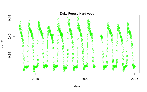
We now have a variety of data related to this ROI from the Hardwood Stand at Duke Forest.
Green Chromatic Coordinate (GCC) is a measure of "greenness" of an area and is
widely used in Phenocam images as an indicator of the green pigment in vegetation.
Let's use this measure to look at changes in GCC over time at this site. Looking
back at the available data, we have several options for GCC. gcc90 is the 90th
quantile of GCC in the pixels across the ROI (for more details,
).
We'll use this as it tracks the upper greenness values while not including many
outliners.
Before we can plot gcc-90 we do need to fix our dates and convert them from
Factors to Date to correctly plot.
# Convert date variable into date format

dukehw_DB_1000[,date:=as.Date(date)]


# plot gcc_90

dukehw_DB_1000[,plot(date, gcc_90, col = 'green', type = 'b')]

#> NULL

mtext('Duke Forest, Hardwood', font = 2)
Download midday images
While PhenoCam sites may have many images in a given day, many simple analyses can use just the midday image when the sun is most directly overhead the canopy. Therefore, extracting a list of midday images (only one image a day) can be useful.
# obtaining midday_images for dukehw

duke_middays <- get_midday_list('dukehw')


# see the first few rows

head(duke_middays)

#> [1] "http://phenocam.nau.edu/data/archive/dukehw/2013/05/dukehw_2013_05_31_150331.jpg"
#> [2] "http://phenocam.nau.edu/data/archive/dukehw/2013/06/dukehw_2013_06_01_120111.jpg"
#> [3] "http://phenocam.nau.edu/data/archive/dukehw/2013/06/dukehw_2013_06_02_120109.jpg"
#> [4] "http://phenocam.nau.edu/data/archive/dukehw/2013/06/dukehw_2013_06_03_120110.jpg"
#> [5] "http://phenocam.nau.edu/data/archive/dukehw/2013/06/dukehw_2013_06_04_120119.jpg"
#> [6] "http://phenocam.nau.edu/data/archive/dukehw/2013/06/dukehw_2013_06_05_120110.jpg"
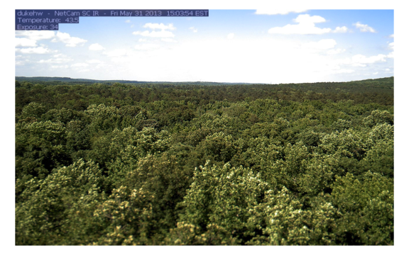
Now we have a list of all the midday images from this Phenocam. Let's download them and plot
# download a file

destfile <- tempfile(fileext = '.jpg')


# download only the first available file

# modify the `[1]` to download other images

download.file(duke_middays[1], destfile = destfile, mode = 'wb')


# plot the image

img <- try(readJPEG(destfile))

if(class(img)!='try-error'){
  par(mar= c(0,0,0,0))
  plot(0:1,0:1, type='n', axes= FALSE, xlab= '', ylab = '')
  rasterImage(img, 0, 0, 1, 1)
}
Download midday images for a given time range
Now we can access all the midday images and download them one at a time. However, we frequently want all the images within a specific time range of interest. We'll learn how to do that next.
# open a temporary directory

tmp_dir <- tempdir()


# download a subset. Example dukehw 2017

download_midday_images(site = 'dukehw', # which site
                       y = 2017, # which year(s)
                       months = 1:12, # which month(s)
                       days = 15, # which days on month(s)
                       download_dir = tmp_dir) # where on your computer


# list of downloaded files

duke_middays_path <- dir(tmp_dir, pattern = 'dukehw*', full.names = TRUE)


head(duke_middays_path)
We can demonstrate the seasonality of Duke forest observed from the camera. (Note this code may take a while to run through the loop).
n <- length(duke_middays_path)

par(mar= c(0,0,0,0), mfrow=c(4,3), oma=c(0,0,3,0))


for(i in 1:n){
  img <- readJPEG(duke_middays_path[i])
  plot(0:1,0:1, type='n', axes= FALSE, xlab= '', ylab = '')
  rasterImage(img, 0, 0, 1, 1)
  mtext(month.name[i], line = -2)
}

mtext('Seasonal variation of forest at Duke Hardwood Forest', font = 2, outer = TRUE)
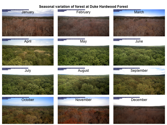
The goal of this section was to show how to download a limited number of midday images from the PhenoCam server. However, more extensive datasets should be downloaded from the .
The most recent release of the phenocamapi R package is available on GitHub: .