AGÕæÈË°Ù¼ÒÀÖ¹Ù·½ÍøÕ¾

This data tutorial provides instruction on working with two different NEON data products to estimate tree height:

• DP3.30015.001, Ecosystem structure, aka Canopy Height Model (CHM)
• DP1.10098.001, Vegetation structure

The are derived from the Lidar point cloud data collected by the remote sensing platform. The are collected by by field staff on the ground. We will be using data from the Wind River Experimental Forest NEON field site located in Washington state. The predominant vegetation there are tall evergreen conifers.

If you are coming to this exercise after following tutorials on data download and formatting, and therefore already have the needed data, skip ahead to section 4.

1. Setup

Start by installing and loading packages (if necessary) and setting options. One of the packages we'll be using, geoNEON, is only available via GitHub, so it's installed using the devtools package. The other packages can be installed directly from CRAN.

Installation can be run once, then periodically to get package updates.

install.packages("neonUtilities")

install.packages("neonOS")

install.packages("terra")

install.packages("devtools")

devtools::install_github("NEONScience/NEON-geolocation/geoNEON")

Now load packages. This needs to be done every time you run code. We'll also set a working directory for data downloads.

library(terra)

library(neonUtilities)

library(neonOS)

library(geoNEON)



options(stringsAsFactors=F)



# set working directory

# adapt directory path for your system

wd <- "~/data"

setwd(wd)

2. Vegetation structure data

Download the vegetation structure data using the loadByProduct() function in the neonUtilities package. Inputs to the function are:

• dpID: data product ID; woody vegetation structure = DP1.10098.001
• site: (vector of) 4-letter site codes; Wind River = WREF
• package: basic or expanded; we'll download basic here
• release: which data release to download; we'll use RELEASE-2023
• check.size: should this function prompt the user with an estimated download size? Set to FALSE here for ease of processing as a script, but good to leave as default TRUE when downloading a dataset for the first time.

Refer to the cheat sheet for the neonUtilities package for more details and the complete index of possible function inputs.

veglist <- loadByProduct(dpID="DP1.10098.001", 
                         site="WREF", 
                         package="basic", 
                         release="RELEASE-2023",
                         check.size = FALSE)

Use the getLocTOS() function in the geoNEON package to get precise locations for the tagged plants. Refer to the package documentation for more details.

vegmap <- getLocTOS(veglist$vst_mappingandtagging, 
                          "vst_mappingandtagging")

Now we have the mapped locations of individuals in the vst_mappingandtagging table, and the annual measurements of tree dimensions such as height and diameter in the vst_apparentindividual table. To bring these measurements together, join the two tables, using the joinTableNEON() function from the neonOS package. Refer to the for Vegetation structure for more information about the data tables and the joining instructions joinTableNEON() is using.

veg <- joinTableNEON(veglist$vst_apparentindividual, 
                     vegmap, 
                     name1="vst_apparentindividual",
                     name2="vst_mappingandtagging")

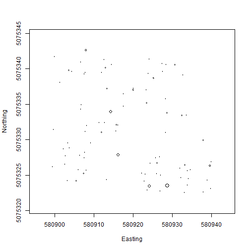
Let's see what the data look like! Make a stem map of the plants in plot WREF_075. Note that the circles argument of the symbols() function expects a radius, but stemDiameter is just that, a diameter, so we will need to divide by two. And stemDiameter is in centimeters, but the mapping scale is in meters, so we also need to divide by 100 to get the scale right.

symbols(veg$adjEasting[which(veg$plotID=="WREF_075")], 
        veg$adjNorthing[which(veg$plotID=="WREF_075")], 
        circles=veg$stemDiameter[which(veg$plotID=="WREF_075")]/100/2, 
        inches=F, xlab="Easting", ylab="Northing")

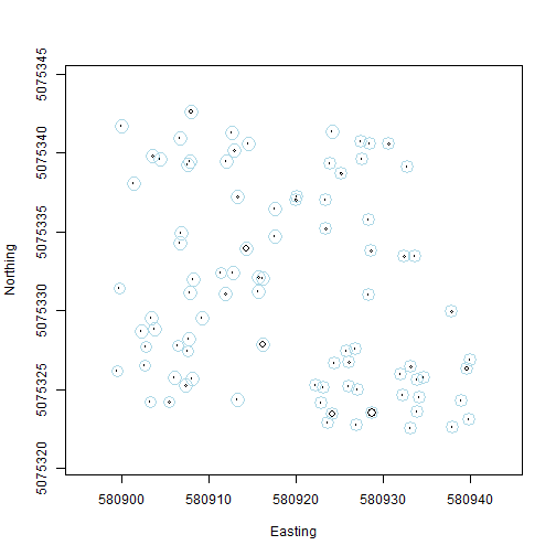
And now overlay the estimated uncertainty in the location of each stem, in blue:

symbols(veg$adjEasting[which(veg$plotID=="WREF_075")], 
        veg$adjNorthing[which(veg$plotID=="WREF_075")], 
        circles=veg$stemDiameter[which(veg$plotID=="WREF_075")]/100/2, 
        inches=F, xlab="Easting", ylab="Northing")

symbols(veg$adjEasting[which(veg$plotID=="WREF_075")], 
        veg$adjNorthing[which(veg$plotID=="WREF_075")], 
        circles=veg$adjCoordinateUncertainty[which(veg$plotID=="WREF_075")], 
        inches=F, add=T, fg="lightblue")

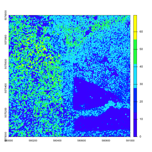
3. Canopy height model data

Now we'll download the CHM tile covering plot WREF_075. Several other plots are also covered by this tile. We could download all tiles that contain vegetation structure plots, but in this exercise we're sticking to one tile to limit download size and processing time.

The tileByAOP() function in the neonUtilities package allows for download of remote sensing tiles based on easting and northing coordinates, so we'll give it the coordinates of all the trees in plot WREF_075 and the data product ID, DP3.30015.001 (note that if WREF_075 crossed tile boundaries, this code would download all relevant tiles).

The download will include several metadata files as well as the data tile. Load the data tile into the environment using the terra package.

byTileAOP(dpID="DP3.30015.001", site="WREF", year="2017", 
          easting=veg$adjEasting[which(veg$plotID=="WREF_075")], 
          northing=veg$adjNorthing[which(veg$plotID=="WREF_075")],
          check.size=FALSE, savepath=wd)



chm <- rast(paste0(wd, "/DP3.30015.001/neon-aop-products/2017/FullSite/D16/2017_WREF_1/L3/DiscreteLidar/CanopyHeightModelGtif/NEON_D16_WREF_DP3_580000_5075000_CHM.tif"))

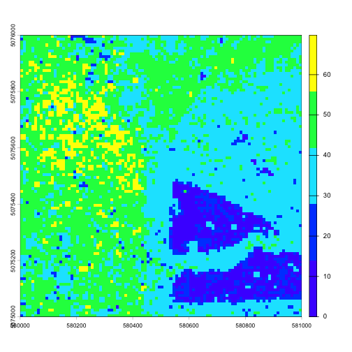
Let's view the tile.

plot(chm, col=topo.colors(5))

4. Comparing the two datasets

Now we have the heights of individual trees measured from the ground, and the height of the top surface of the canopy, measured from the air. There are many different ways to make a comparison between these two datasets! This section will walk through three different approaches.

First, subset the vegetation structure data to only the trees that fall within this tile, using the ext() function from the terra package.

This step isn't strictly necessary, but it will make the processing faster.

vegsub <- veg[which(veg$adjEasting >= ext(chm)[1] &
                      veg$adjEasting <= ext(chm)[2] &
                      veg$adjNorthing >= ext(chm)[3] & 
                      veg$adjNorthing <= ext(chm)[4]),]

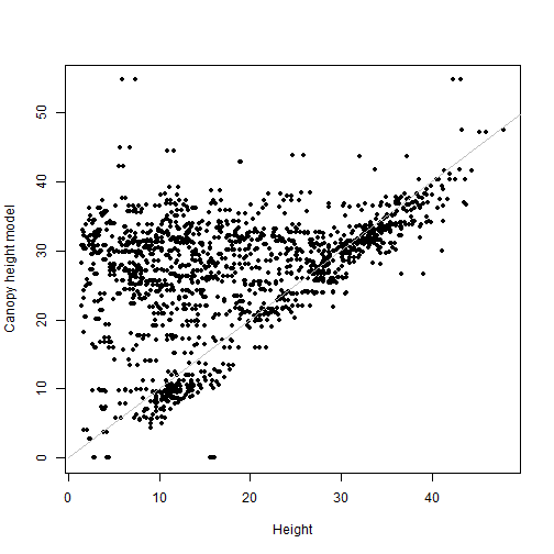
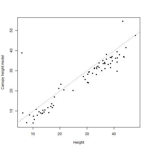
Starting with a very simple first pass: use the extract() function from the terra package to get the CHM value matching the coordinates of each mapped plant. Then make a scatter plot of each tree's height vs. the CHM value at its location.

valCHM <- extract(chm, 
                  cbind(vegsub$adjEasting,
                  vegsub$adjNorthing))



plot(valCHM$NEON_D16_WREF_DP3_580000_5075000_CHM~
       vegsub$height, pch=20, xlab="Height", 
     ylab="Canopy height model")

lines(c(0,50), c(0,50), col="grey")

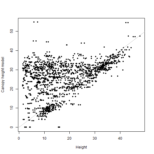
How strong is the correlation between the ground and lidar measurements?

cor(valCHM$NEON_D16_WREF_DP3_580000_5075000_CHM, 
    vegsub$height, use="complete")

## [1] 0.3824467

Now we remember there is uncertainty in the location of each tree, so the precise pixel it corresponds to might not be the right one. Let's try adding a buffer to the extraction function, to get the tallest tree within the uncertainty of the location of each tree.

valCHMbuff <- extract(chm, 
                  buffer(vect(cbind(vegsub$adjEasting,
                  vegsub$adjNorthing)),
                  width=vegsub$adjCoordinateUncertainty),
                  fun=max)



plot(valCHMbuff$NEON_D16_WREF_DP3_580000_5075000_CHM~
       vegsub$height, pch=20, xlab="Height", 
     ylab="Canopy height model")

lines(c(0,50), c(0,50), col="grey")

cor(valCHMbuff$NEON_D16_WREF_DP3_580000_5075000_CHM, 
    vegsub$height, use="complete")

## [1] 0.3698753

Adding the buffer has actually made our correlation slightly worse. Let's think about the data.

There are a lot of points clustered on the 1-1 line, but there is also a cloud of points above the line, where the measured height is lower than the canopy height model at the same coordinates. This makes sense, because the tree height data include the understory. There are many plants measured in the vegetation structure data that are not at the top of the canopy, and the CHM sees only the top surface of the canopy.

This also explains why the buffer didn't improve things. Finding the highest CHM value within the uncertainty of a tree should improve the fit for the tallest trees, but it's likely to make the fit worse for the understory trees.

How to exclude understory plants from this analysis? Again, there are many possible approaches. We'll try out two, one map-centric and one tree-centric.

Starting with the map-centric approach: select a pixel size, and aggregate both the vegetation structure data and the CHM data to find the tallest point in each pixel. Let's try this with 10m pixels.

Start by rounding the coordinates of the vegetation structure data, to create 10m bins. Use floor() instead of round() so each tree ends up in the pixel with the same numbering as the raster pixels (the rasters/pixels are numbered by their southwest corners).

easting10 <- 10*floor(vegsub$adjEasting/10)

northing10 <- 10*floor(vegsub$adjNorthing/10)

vegsub <- cbind(vegsub, easting10, northing10)

Use the aggregate() function to get the tallest tree in each 10m bin.

vegbin <- stats::aggregate(vegsub, 
                           by=list(vegsub$easting10, 
                                   vegsub$northing10), 
                           FUN=max)

To get the CHM values for the 10m bins, use the terra package version of the aggregate() function. Let's take a look at the lower-resolution image we get as a result.

CHM10 <- terra::aggregate(chm, fact=10, fun=max)

plot(CHM10, col=topo.colors(5))

Use the extract() function again to get the values from each pixel. Our grids are numbered by the corners, so add 5 to each tree coordinate to make sure it's in the correct pixel.

vegbin$easting10 <- vegbin$easting10 + 5

vegbin$northing10 <- vegbin$northing10 + 5

binCHM <- extract(CHM10, cbind(vegbin$easting10, 
                               vegbin$northing10))

plot(binCHM$NEON_D16_WREF_DP3_580000_5075000_CHM~
       vegbin$height, pch=20, 
     xlab="Height", ylab="Canopy height model")

lines(c(0,50), c(0,50), col="grey")

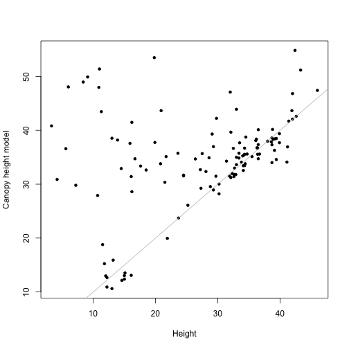
cor(binCHM$NEON_D16_WREF_DP3_580000_5075000_CHM, 
    vegbin$height, use="complete")

## [1] 0.2244228

The understory points are thinned out substantially, but so are the rest. We've lost a lot of data by going to a lower resolution.

Let's try and see if we can identify the tallest trees by another approach, using the trees as the starting point instead of map area. Start by sorting the veg structure data by height.

vegsub <- vegsub[order(vegsub$height, 
                       decreasing=T),]

Now, for each tree, let's estimate which nearby trees might be beneath its canopy, and discard those points. To do this:

1. Calculate the distance of each tree from the target tree.
2. Pick a reasonable estimate for canopy size, and discard shorter trees within that radius. The radius I used is 0.3 times the height, based on some rudimentary googling about Douglas fir allometry. It could definitely be improved on!
3. Iterate over all trees.

We'll use a simple for loop to do this:

vegfil <- vegsub

for(i in 1:nrow(vegsub)) {
    if(is.na(vegfil$height[i]))
        next
    dist <- sqrt((vegsub$adjEasting[i]-vegsub$adjEasting)^2 + 
                (vegsub$adjNorthing[i]-vegsub$adjNorthing)^2)
    vegfil$height[which(dist<0.3*vegsub$height[i] & 
                        vegsub$height<vegsub$height[i])] <- NA
}



vegfil <- vegfil[which(!is.na(vegfil$height)),]

Now extract the raster values, as above.

filterCHM <- extract(chm, 
                     cbind(vegfil$adjEasting, 
                           vegfil$adjNorthing))

plot(filterCHM$NEON_D16_WREF_DP3_580000_5075000_CHM~
       vegfil$height, pch=20, 
     xlab="Height", ylab="Canopy height model")

lines(c(0,50), c(0,50), col="grey")

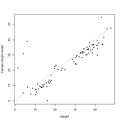
cor(filterCHM$NEON_D16_WREF_DP3_580000_5075000_CHM,
    vegfil$height)

## [1] 0.8070586

This is quite a bit better! There are still several understory points we failed to exclude, but we were able to filter out most of the understory without losing so many overstory points.

Let's try one last thing. The plantStatus field in the veg structure data indicates whether a plant is dead, broken, or otherwise damaged. In theory, a dead or broken tree can still be the tallest thing around, but it's less likely, and it's also less likely to get a good Lidar return. Exclude all trees that aren't alive:

vegfil <- vegfil[which(vegfil$plantStatus=="Live"),]

filterCHM <- extract(chm, 
                     cbind(vegfil$adjEasting, 
                           vegfil$adjNorthing))

plot(filterCHM$NEON_D16_WREF_DP3_580000_5075000_CHM~
       vegfil$height, pch=20, 
     xlab="Height", ylab="Canopy height model")

lines(c(0,50), c(0,50), col="grey")

cor(filterCHM$NEON_D16_WREF_DP3_580000_5075000_CHM,
    vegfil$height)

## [1] 0.9057883

Nice!

One final note: however we slice the data, there is a noticeable bias even in the strongly correlated values. The CHM heights are generally a bit shorter than the ground-based estimates of tree height. There are two biases in the CHM data that contribute to this. (1) Lidar returns from short-statured vegetation are difficult to distinguish from the ground, so the "ground" estimated by Lidar is generally a bit higher than the true ground surface, and (2) the height estimate from Lidar represents the highest return, but the highest return may slightly miss the actual tallest point on a given tree. This is especially likely to happen with conifers, which are the top-of-canopy trees at Wind River.